Machine Learning for Time Series
Contents
- Introduction
- Time Series Classification
- Time Series Forecasting
- Time Series Clustering
- Anomaly Detection
- Multi-task Models: Hidden Markov Models
- Other Time Series Machine Learning Tasks
- Applications
- Useful Resources for Time Series Analysis
- References
Due to their natural temporal ordering, time series data are present in almost every task that requires some sort of human cognitive process. Industries varying from health care, remote sensing and aerospace engineering all now produce time series datasets of previously unseen scale. Due to that, the different machine learning tasks associated to time series, such as time series classification, time series forecasting and anomaly detection have been considered as one of the most challenging problems in the field during the last decade. In comparison to the fields of computer vision and natural language processing, the increasing use of time series has not been met with a complete adoption of deep learning-based approaches during the last five years, and thus, their analysis is approached from different perspectives. In this section, the basics of the main machine learning tasks with time series data will be reviewed, along with the different approaches developed to tackle them.
Introduction
A time series $X$ is an ordered sequence of t real values $X = {x_1, . . . , x_t}$, $x_i \in R$, $i \in N$.
Due to their natural temporal ordering, time series data are present in almost every task that requires some sort of human cognitive process.
Time series are encountered in many real-world applications ranging from:
- Electronic health records
- Human activity recognition
- Cybersecurity
- Aerospace Engineering
When analysing a dataset of time series data, there are multiple characteristics that one must check before choosing a technique:
- Type of data contained in the time series
- Number of variables
- Time series length
- Spacing of observation times
- Presence of missing values
- Stationarity
Type of data
In the literature, the keyword time series usually refers to countinuous data, while the keyword sequence usually refers to categorical data (symbols).
Number of variables
Classic datasets of time series are normally univariate. However, the increase amount of sensor data available in different domains is increasing the need of analysis of multivariate time series.
Time series length
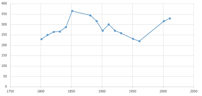
Research into time series classification has tended to focus on the case of series of uniform length. However, it is common for real-world time series data to have unequal lengths.
Spacing of observation times
As opposed to evenly (or regular) spaced time series, in (or irregular) the spacing of observation times is not constant.

Stationarity
A stationary time series is one whose statistical properties such as the mean, variance and autocorrelation are all constant over time. Non-stationary data should be first converted into stationary data in some classic modelling techniques such as ARMA.

Machine learning tasks for time series analysis
Time Series Classification
Time Series Classification (TSC) is a supervised learning problem that aims to predict a discrete label y $\in$ {1, $\dots$, c} for an unlabeled time series, where c is the number of classes in the TSC task.
UCR/UEA archive
The UCR time series archive [1] is the defacto standard in TSC research for benchmarking algorithms. It contains up to 128 time series datasets from several application domains:
- All of the time series are univariate.
- No missing values are present.
- No irregular time series.
- No varying length time series.
A more recent benchmarking tool is the UEA archive [2], which gathers multivariate time series datasets for benchmarking algorithms.
The techniques for TSC can be broadly categorized into different classes. Here we will focus on:
- Similarity-based techniques
- Feature-based techniques
- Deep learning-based techniques
- Bag of Words techniques
Similarity-based techniques
These algorithms usually use 1-Nearest Neighbour (1-NN) with elastic similarity measures. Elastic measures are designed to compensate for local distortions, miss-alignments or warpings in time series that might be due to stretched or shrunken subsections within the time series.
Commonly used similarity measures include:
- Dynamic Time Warping (DTW) [3]
- Longest Common Subsequence (LCSS) [4]
- Move-Split-Merge (MSM) [5]
- Time Warp Edit Distance (TWE) [6]
Ensembles formed using multiple 1-NN classifiers with a diversity of similarity measures have proved to be significantly more accurate than 1-NN with any single measure [7].
Feature-based techniques
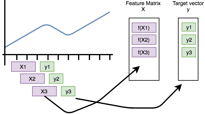
Calculate different characteristics (features) from substructures of the time series and use them to compare and classify them.
The extracted features can be used to build models that perform classification/regression tasks on the time series. These methods transform the time series into a set of features, transforming the dataset into a tabular format, suitable for classic machine learning.
Many of the successul feature extraction techniques for time series are domain specific and require expert knowledge, such as:
- Features from Electrocardiogram (ECG).
- Features from acoustic signals (spectogram).

However, there are different libraries to automatically extract a relevant set of features from a dataset of time series:
- tsfresh: A Python package that computes a total of 794 time series features, with feature selection on basis automatically configured hypothesis tests. [8] (code)
- tsfeatures: A R package that provides methods for extracting various features from time series data. (code)
- ROCKET (2019): Random convolutional kernels are used to capture discriminative patterns in the time series data. [9] (code)
Deep learning for TSC
Since the recent success of deep learning techniques in supervised learning such as image recognition and natural language processing, researchers started investigating these complex ma- chine learning models for TSC.
Precisely, Convolutional Neural Networks (CNNs) have showed promising results for TSC.
Given an input time series, a convolutional layer consists of sliding one-dimensional filters over the time series, thus enabling the network to extract non-linear discriminant features that are time-invariant and useful for classification. The filter can also be seen as a generic non-linear transformation of a time series.

By cascading multiple convolutional layers, the network is able to further extract hierarchical features that should in theory improve the network’s prediction.

Some popular deep learning architectures for TSC are:
- ResNet: A deep CNN coupled with residual connections, following the sucessful ideas applied in computer vision. [10] [code]
- InceptionTime: An ensemble of five deep learning models for TSC. [11] [code]
Other TSC Strategies: Imaging Time Series
There are some transformation algorithms, such as Gramian Angular Difference Field, that transform time series into images, and then apply the powerful advances of transfer learning in computer vision for classifying those images.

Classification for Class-Imbalanced Data
See Machine Learning using Class-Imbalanced Data
Time Series Forecasting
In forecasting, the machine predicts future time series based on past observed data. The better the interdependencies among different series are modeled, the more accurate the forecasting can be.

The most well-known model for linear univariate time series forecasting are:
- AutoRegressive Integrated Moving Average (ARIMA) [12], which relies heavily on correlations (and partial autocorrelation) patterns in the data.
- Linear Support Vector Regression (SVR) [13], which treats the forecasting problem as a typical regression problem with time-varying parameters.
However, these models are mostly limited to linear univariate time series and do not scale well to multivariate time series.
To forecast multivariate time series, classic approaches are:
- Vector AutoRegression (VAR) [12], a generalization of AutoRegression models.
- Gaussian Processes (GP) [14].
Still, these approaches apply predetermined non-linearities and may fail to recognize different forms of non-linearity.
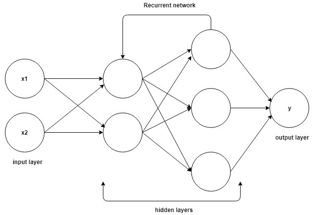
Recently, deep neural networks, more specifically, Recurrent Neural Networks and Long Short Term Memory (LSTM) architectures have received great amount of attention due to they present loops in the connections between neurons, which give the ability to capture non-linear interdependencies [15], [16].
A common LSTM unit is composed of a cell, an input gate, an output gate and a forget gate. The cell remembers values over arbitrary time intervals and the three gates regulate the flow of information into and out of the cell.
Time Series Clustering
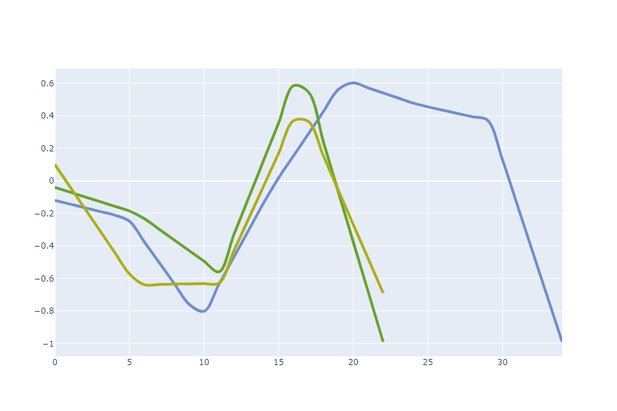
Time series clustering is an unsupervised machine learning task. The goal is to divide a set of time series into groups, according to a pre-defined distance or similarity measure. Results are usually displayed in a dendogram, which shows the hierarchical relationship between the time series in the dataset.

Clustering Configuration
In order to perform time series clustering, three important hyperparameters need to be fixed:
- the dissimilarity measure: The R package TSDist gathers a set of commonly used distance measures that can be used to measure the dissimilarity between time series.
- the clustering method: Most common classic ones are K-means [ref], K-medoids [17] and DBSCAN [18].
- the number of clusters: Some algorithms decide this value automatically (e.g. DBSCAN).
External Validation
External measures are applicable when there is prior knowledge (ground truth, labels) about the data:
- Rand statistic
- Jaccard coefficient
- $\dots$
See here for more information about these measures.
Internal Validation
When there are no labels in the data, the results of a clustering algorithm must be assessed by an internal validation indices, such as the silhouette width [19], that ensure:
- Cohesion: measures how closely related objects are in a cluster.
- Separation: measures how distinct a cluster is from other clusters.
When there is no prior information about the different groups in which each performance measure can be discriminated, different clustering solutions are computed values for different hyperparameter sets:
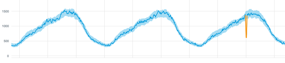
Anomaly Detection
An anomaly is usually defined as points in certain time steps where the system’s behaviour is significantly different from the previous normal status. The basic task of anomaly detection is thus to identify the time steps in which an anomaly may have occurred.Given the inherent lack of labeled anomaly data for training supervised algorithms, anomaly detection methods are mostly based on unsupervised methods.
Some general unsupervised anomaly detection methods that can also be applied to (multivariate) time series are:
- Linear model-based methods [20]: Based on Principal Component Analysis (PCA), they are only effective for highly correlated data, and require the data to follow multivariate Gaussian distribution.
- Distance-based methods [21], [22]: Based on KNN and outlier detection through clustering. Although effective in some cases, these distance-based methods perform better with priori knowledge about anomaly durations and the number of anomalies.
Deep Learning-Based Methods
Recent promising results focus on the basis of the Generative Adversarial Networks (GAN). One example is MAD-GAN [23] [code], which adopts the Long Short Term-Recurrent Neural Networks (LSTM-RNN) as the base models learned by the GAN to capture the temporal dependency in multivariate time series.
Multi-Task Models: Hidden Markov Models
Some models, such as Hidden Markov Models (HMMs) provide an unified way of extracting patterns from sequential data, and then use them for:
- Pattern analysis
- Classification
- Clustering
- Forecasting

HMMs for Interpreting Patterns
Each state in the model represents a high level pattern, given by the probability distribution of the low levels sequential data feeding the model. Those states are linked by a Markov chain.

HMMs for Time Series Classification
The time series of each class are used to fit a different HMM. Then, when a test data is presented, the model whose probability of generating the test sequence is higher will be chosen as the predicted class.
Other Time Series Machine Learning Tasks
Representation Learning for High Dimensional Time Series
Since human cognition is not optimized to work well in high-dimensional spaces, these areas could benefit from interpretable low-dimensional representations. However, most algorithms for time series data are difficult to interpret. This is due to non-intuitive mappings from data features to salient properties of the representation and non-smoothness over time. To address this problem, representation learning algorithms allow to approximate a high dimensional countinuos space of time series with a lower dimensional discrete one.
Learning discrete representations of high-dimensional time series give rise to smooth and interpretable embeddings with superior clustering performance. Some popular representation learning algorithms are:
Time Series Cross-Validation
Cross-validation (CV) is a popular technique for tuning hyperparameters by iteratively training the model on a training and validation subset of the data before the model performance can be measured on the final testing set.
However, issues arise when applying this technique in the case of time series data [27]:
- Care must be taken when splitting the data into subsets due to it´s inherent time dependence (to avoid data leakage).
- To avoid an arbitrary splitting of the initial data that may lead to a poor result on an independent test set, a technique called Nested CV should be used which introduces a secondary iterative process over the splitting itself.
Possible Nested CV algorithms for both single, and multiple independent time series are discussed here.
Time Series Imputation
Many analysis methods require missing values to be replaced with reasonable values up-front. In statistics this process of replacing missing values is called imputation.
The R package imputeTS offers multiple state-of-the-art imputation techniques:


Scaling
Scaling refers to how we prepare the data so that the network can really leverage all the information it contains.
There are 2 main types of scaling:
- standardize: where you process your data to get to a mean of 0 and standard deviation of 1
- normalize: where you process your data to be within a range (usually -1, 1)
Each of these 2 types have 3 subtypes:
- all samples: where you extract the statistics that you will then apply from all train samples at the same time (1 mean and 1 std or 1 min and 1 max).
- (all samples) per channel: where you extract the statistics that you will then apply from each channel of all train samples (1 mean and 1 std or 1 min and 1 max per channel).
- per sample: here you just calculate the stats for each individual sample, and then process each sample individually.
Applications
See here for examples of the above techniques applied to Space.
Useful Resources for Time Series Analysis
Python libraries/repositories for time series
- pyts: Focused on time series classification, this package gathers many of the state of the art for both univariate and multivariate time series, with the exception of deep learning-based ones.
- tslearn: Built on top of
scikit-learn, this package provides tools for a variety of machine learning tasks, as well as preprocessing methods. - timeSeriesAI: This repository is focused on deep learning for time series classification using the fastai deep learning library. It contains step by step Jupyter notebooks showing how to apply cutting edge research on TSC to your data.
- prophet : Tool for producing high quality forecasts. Made by Facebook’s Data Science Team. R and Python Interfaces.
- gluon-ts: Probabilistic Time Series Modeling in Python
R libraries for time series
- xts: Extensible Time Series: Provide for uniform handling of R’s different time-based data classes.
- forecast: Provides a collection of commonly used univariate and multivariate time series forecasting models including exponential smoothing via state space models and automatic ARIMA modelling.
- TSclust: A set of measures of dissimilarity between time series to perform time series clustering.
Annotation/Labelling of Time Series
Labeled data (also known as the ground truth) is necessary for evaluating time series machine learning. Otherwise, one can not easily choose a detection method, or say method A is better than method B. The labeled data can also be used as the training set if one wants to develop supervised learning methods for detection.
Annotation tools provide visual ways to:
- Mark time windows with the presence of anomalies in time series
- Give categories (classes) to time series
Annotation tools
- Curve - Curve is an open-source tool to help label anomalies on time-series data
- TagAnomaly - Anomaly detection analysis and labeling tool, specifically for multiple time series (one time series per category)
- time-series-annotator - The CrowdCurio Time Series Annotation Library implements classification tasks for time series.
- WDK - The Wearables Development Toolkit (WDK) is a set of tools to facilitate the development of activity recognition applications with wearable devices.
- Label Studio - Label Studio is a configurable data annotation tool that works with different data types
References
[1]: Dau H.A., Bagnall A., et al. (2019), The UCR Time Series Archive. arXiv:1810.07758v2
[2]: Bagnall A., Dau H.A., et al. (2018), The UEA multivariate time series classification archive, 2018. arXiv:1811.00075
[3]: Jeong, Y. S., Jeong, M. K., & Omitaomu, O. A. (2011). Weighted dynamic time warping for time series classification. In Pattern Recognition (Vol. 44, pp. 2231–2240). https://doi.org/10.1016/j.patcog.2010.09.022
[4]: Hirschberg, D. S. (1977). Algorithms for the Longest Common Subsequence Problem. Journal of the ACM (JACM), 24(4), 664–675. https://doi.org/10.1145/322033.322044
[5]: Stefan, A., Athitsos, V., & Das, G. (2013). The move-split-merge metric for time series. IEEE Transactions on Knowledge and Data Engineering, 25(6), 1425–1438. https://doi.org/10.1109/TKDE.2012.88
[6]: Marteau, P. F. (2009). Time warp edit distance with stiffness adjustment for time series matching. IEEE Transactions on Pattern Analysis and Machine Intelligence, 31(2), 306–318. https://doi.org/10.1109/TPAMI.2008.76
[7]: Lucas, B., Shifaz, A., Pelletier, C., O’Neill, L., Zaidi, N., Goethals, B., … Webb, G. I. (2019). Proximity Forest: an effective and scalable distance-based classifier for time series. Data Mining and Knowledge Discovery, 33(3), 607–635. https://doi.org/10.1007/s10618-019-00617-3
[8]: Christ, M., Braun, N., Neuffer, J., & Kempa-Liehr, A. W. (2018). Time Series FeatuRe Extraction on basis of Scalable Hypothesis tests (tsfresh – A Python package). Neurocomputing, 307, 72–77. https://doi.org/10.1016/j.neucom.2018.03.067
[9]: Dempster A., Petitjean F., Webb G. (2019). ROCKET: Exceptionally fast and accurate time series classification using random convolutional kernels. arXiv:1910.13051
[10]: Ismail Fawaz, H., Forestier, G., Weber, J., Idoumghar, L., & Muller, P. A. (2019). Deep learning for time series classification: a review. Data Mining and Knowledge Discovery, 33(4), 917–963. https://doi.org/10.1007/s10618-019-00619-1
[11]: Fawaz H., Lucas B., Forestier G., et al. (2019). InceptionTime: Finding AlexNet for Time Series Classification. arXiv:1909.04939
[12]: Box G., Jenkins G., Reinsel G., et al. (2015). Time Series Analysis: Forecasting and Control, 5th Edition. ISBN: 978-1-118-67502-1
[13]: Cao, L. J., & Tay, F. E. H. (2003). Support vector machine with adaptive parameters in financial time series forecasting. IEEE Transactions on Neural Networks, 14(6), 1506–1518. https://doi.org/10.1109/TNN.2003.820556
[14]: Frigola R., Rasmussen C. (2013). Integrated Pre-Processing for Bayesian Nonlinear System Identification with Gaussian Processes, Proceedings of the 52th IEEE International Conference on Decision and Control (CDC), Firenze, Italy, December 2013. arXiv:1303.2912
[15]: Lai G., Chang W., Yang Y., et al. (2017). Modeling Long- and Short-Term Temporal Patterns with Deep Neural Networks. arXiv:1703.07015
[16]: Shih S., Sun F., Lee H. (2018). Temporal Pattern Attention for Multivariate Time Series Forecasting. arXiv:1809.04206
[17]: Park, H. S., & Jun, C. H. (2009). A simple and fast algorithm for K-medoids clustering. Expert Systems with Applications, 36(2 PART 2), 3336–3341. https://doi.org/10.1016/j.eswa.2008.01.039
[18]: Ester, M., Kriegel, H.-P., Sander, J., & Xu, X. (1996). A Density-Based Algorithm for Discovering Clusters in Large Spatial Databases with Noise. In Proceedings of the 2nd International Conference on Knowledge Discovery and Data Mining (pp. 226–231). Portland, OR, USA. AAAI
[19]: Rousseeuw, P. J. (1987). Silhouettes: A graphical aid to the interpretation and validation of cluster analysis. Journal of Computational and Applied Mathematics, 20(C), 53–65. https://doi.org/10.1016/0377-0427(87)90125-7
[20]: Li, S., & Wen, J. (2014). A model-based fault detection and diagnostic methodology based on PCA method and wavelet transform. Energy and Buildings, 68(PARTA), 63–71. https://doi.org/10.1016/j.enbuild.2013.08.044
[21]: Angiulli, F., & Pizzuti, C. (2002). Fast outlier detection in high dimensional spaces. In Lecture Notes in Computer Science (including subseries Lecture Notes in Artificial Intelligence and Lecture Notes in Bioinformatics) (Vol. 2431 LNAI, pp. 15–27). https://doi.org/10.1007/3-540-45681-3_2
[22]: Breuniq, M. M., Kriegel, H. P., Ng, R. T., & Sander, J. (2000). LOF: Identifying density-based local outliers. SIGMOD Record (ACM Special Interest Group on Management of Data), 29(2), 93–104. https://doi.org/10.1145/335191.335388
[23]: Li, D., Chen, D., Jin, B., Shi, L., Goh, J., & Ng, S. K. (2019). MAD-GAN: Multivariate Anomaly Detection for Time Series Data with Generative Adversarial Networks. In Lecture Notes in Computer Science (including subseries Lecture Notes in Artificial Intelligence and Lecture Notes in Bioinformatics) (Vol. 11730 LNCS, pp. 703–716). Springer Verlag. https://doi.org/10.1007/978-3-030-30490-4_56
[24]: Kohonen, T. (1990). The Self-Organizing Map. Proceedings of the IEEE, 78(9), 1464–1480. https://doi.org/10.1109/5.58325
[26]: Fortuin, V., Hueser, M., Locatello, F., Strathmann, H., & Rätsch, G. (2019). Som-Vae: Interpretable discrete representation learning on time series. In 7th International Conference on Learning Representations, ICLR 2019. International Conference on Learning Representations, ICLR. arXiv:1806.02199
[27]: Varma S., Simon R. (2006). Bias in error estimation when using cross-validation for model selection. BMC Bioinformatics, 7(1):91. ISSN 1471–2105. doi: 10.1186/1471–2105-7-91
Image Credits
- Multivariate time series with unequal lengths
- Illustration of even vs uneven data frequency
- Example of stationary vs non-stationary time series
- Underlying features in time series may be used to compare datasets
- Features present in an electrocardiogram signal
- Illustration of resultant features using convolutions
- Architecture of a Convolutional Neural Network
- Model trained on historic blue data and used to predict future pink
- Recurrent Neural Network Architecture
- Dendogram: Characteristic-based Clustering for Time Series Data
- Time series (blue) with detectable anomaly (orange)
- Interpolation of missing values using different strategies
- Annotation tool for classifying time series