The Sun-shadow dynamics
The solar radiation pressure can be a significant perturbation for the motion of Earth satellites which have area to mass ratio large enough, such as the Echo balloons [Parkinson et al., 1960]. However, it has no effects in the Earth shadow region. To study the short-period evolution of an Earth satellite which is periodically eclipsed by the Earth, we introduce the Sun-shadow dynamics, following the idea in [Beletski, 2001]: we assume Kepler’s dynamics inside the Earth shadow, and Stark’s dynamics outside of it.
In the following, we consider the two-dimensional case where the solar radiation pressure force lies in the plane of motion of the satellites. Before investigating the alternation of the two different dynamics, we introduce Kepler’s and Stark’s dynamics and a set of suitable coordinates which are separables for the Hamilton-Jacobi equations of both the two problems; we also revise some main feautures of Stark’s planar trajectories. Then, for a further description of the Sun-shadow dynamics, a Poincaré-like map called Sun-shadow map is defined and analysed. For additional details on the subject, refer to [Cavallari, Gronchi, Baù, 2020].
Table of Contents
Kepler’s and Stark’s dynamics
Kepler’s dynamics is defined by
\[\ddot{\boldsymbol{x}} = -\frac{\mu\boldsymbol{x}}{|\boldsymbol{x}|^3}\]where $\mu$ is the Earth gravitation parameter and $\boldsymbol{x}=(x,y)\in \mathbb{R}^2$. The corresponding Hamiltonian function is
\[H_k = \frac{1}{2}(p_x^2+p_y^2) - \frac{\mu}{\sqrt{x^2+y^2}},\]where $p_x, p_y$ are the momenta conjugated to $x,y$. Besides $H_k$, Kepler’s problem has further first integrals, which are the angular momentum
\[C_k = p_y x - p_x y\]and the Laplace-Lenz vector
\[\boldsymbol{A}_k = \left( \begin{aligned} &p_y(p_y x - p_x y) - \frac{\mu x}{\sqrt{x^2+y^2}}\\ &p_x(p_xy - p_yx) - \frac{\mu y}{\sqrt{x^2+y^2}}\\ \end{aligned} \right).\]In the following, the opposite of the $x$-component of $\boldsymbol{A}_k$ is denoted by $L_k$ .
On the other hand, Stark’s dynamics is given by
\[\ddot{\boldsymbol{x}} = -\frac{\mu\boldsymbol{x}}{|\boldsymbol{x}|^3} + f\boldsymbol{e_1}, \qquad f>0\]where $\boldsymbol{e_1}$ is a unit vector aligned with the $x$ axis and its Hamiltonian function is
\[H_s = \frac{1}{2}(p_x^2+p_y^2) - \frac{\mu}{\sqrt{x^2+y^2}} - fx.\]Stark’s two-dimensional dynamics has only one further integral independent from $H_s$, given by
\[L_s = p_y(p_x y - p_y x) + \frac{\mu x}{\sqrt{x^2+y^2}} - \frac{f}{2}y^2,\]which is a generalisation of $L_k$ (see [Redmond, 1964]).
By means of the canonical transformation $(p_x,p_y,x,y)\mapsto (p_u,p_v,u,v)$ defined by
\[\begin{aligned} x =& \frac{u^2-v^2}{2},\\ y =& uv,\\ p_x =& \frac{p_u u-p_v v}{u^2+v^2},\\ p_y =& \frac{p_uv+p_vu}{u^2+v^2}, \\ \end{aligned}\]we introduce variables which are separated in the Hamilton-Jacobi equations for both Kepler’s and Stark’s problems.
It is also useful to perform a transformation of the time variable $t$ and introduce then the fictitious time $\tau$ through relation
\[\frac{d\tau}{dt}= \frac{1}{u^2+v^2}.\]Hamilton’s functions of Kepler’s and Stark’s problems in the new variables are
\[\begin{align} \mathscr{H}_k &= \frac{p_u^2+p_v^2}{2(u^2+v^2)} - \frac{2\mu}{u^2+v^2}, \\ \mathscr{H}_s &= \frac{p_u^2+p_v^2}{2(u^2+v^2)} - \frac{2\mu}{u^2+v^2} - \frac{f}{2}(u^2-v^2); \\ \end{align}\]the integrals $L_k,L_s$ become
\[\begin{align} \mathscr{L}_k &= \frac{p_u^2v^2 - p_v^2u^2}{2(u^2+v^2)} + \mu\frac{u^2-v^2}{u^2+v^2}, \\ \mathscr{L}_s &= \frac{p_u^2v^2 - p_v^2u^2}{2(u^2+v^2)} + \mu\frac{u^2-v^2}{u^2+v^2} - \frac{f}{2}u^2v^2. \\ \end{align}\]The Hamilton-Jacobi equation for Kepler’s problem is
\[\biggl(\frac{\partial W_k}{\partial u}\biggr)^2+\biggl(\frac{\partial W_k}{\partial v}\biggr)^2 = 2\bigl(h_k(u^2+v^2) + 2\mu\bigr),\]where $h_k$ is the value of $\mathscr{H}_k$ for some given initial condition and $W_k$ is the unknown generating function.
Similarly, the Hamilton-Jacobi equation for Stark’s problem is
\[\biggl(\frac{\partial W_s}{\partial u}\biggr)^2+\biggl(\frac{\partial W_s}{\partial v}\biggr)^2 = 2\bigl(h_s(u^2+v^2) + 2\mu\bigr) + f(u^4-v^4),\]with $h_s$ the value of $\mathscr{H}_s$ and $W_s$ the unknown generating function. As anticipared, in both the two previous equations the variables are separated. Thus, for Kepler’s dynamics it holds
\[\left\{ \begin{aligned} &p_u^2 - 2(h_k u^2 + \mu) = \alpha_k,\\ &p_v^2 - 2(h_k v^2 + \mu) = -\alpha_k,\\ \end{aligned} \right. .\]If we substitute the expressions of $p_u^2$ and $p_v^2$ given by these relations into equation
\[\mathscr{L}_k(p_u,p_v,u,v) = \ell_k\]with $\ell_k$ a value of $\mathscr{L}_k$, we obtain that the integration constant $\alpha_k$ is equal to
\[\alpha_k = 2 \ell_k.\]Similarly, for Stark’s dynamics we get
\[\left\{ \begin{aligned} &p_u^2 - \bigl(2(h_s u^2 + \mu) + fu^4\bigr) = \alpha_s,\\ &p_v^2 - \bigl(2(h_s v^2 + \mu) - fv^4\bigr) = -\alpha_s,\\ \end{aligned} \right.\]where
\[\alpha_s = 2\ell_s,\]with $\ell_s$ a value of $\mathscr{L}_s$.
Stark’s trajectories
In [Beletski, 1964], Beletsky shows that all the possible planar trajectories of Stark’s problem can be classified into four categories, depending on the values $\ell_s,h_s$ of the integrals $\mathscr{L}_s,\mathscr{H}_s$.
Since
\[\begin{aligned} & p_u^2 = U(u), \qquad U(u) = fu^4+2h_s u^2+2(\mu+\ell_s),\\ & p_v^2=V(v), \qquad V(v) = -fv^4+2h_s v^2+2(\mu-\ell_s),\\ \end{aligned}\]to have real values of \(p_u\) and \(p_v\) we must fulfil the conditions
\[U(u)\geq 0, \qquad V(v)\geq 0,\]which restrict the possible configurations depending on the values $\ell_s$, $h_s$.
By setting
\[\xi = u^2, \qquad \eta = v^2,\]we can write the polynomials $U(u)$ and $V(v)$ as follows
\[U(u)= f(\xi-\xi_1)(\xi-\xi_2),\qquad V(v)= -f(\eta-\eta_1)(\eta-\eta_2),\]with
\[\begin{aligned} &\xi_1 = -\frac{h_s}{f}+\sqrt{\frac{h_s^2}{f^2}-\frac{2(\mu+\ell_s)}{f}}, \qquad \xi_2 = -\frac{h_s}{f}-\sqrt{\frac{h_s^2}{f^2}-\frac{2(\mu+\ell_s)}{f}},\\ &\eta_1 = \frac{h_s}{f}+\sqrt{\frac{h_s^2}{f^2}+\frac{2(\mu-\ell_s)}{f}}, \qquad \eta_2 = \frac{h_s}{f}-\sqrt{\frac{h_s^2}{f^2}+\frac{2(\mu-\ell_s)}{f}}.\\ \end{aligned}\]Denoting
\[{u}_1 = \sqrt{\xi_1}, \qquad {u}_2 = \sqrt{\xi_2},\qquad {v}_1 = \sqrt{\eta_1}, \qquad {v}_2 = \sqrt{\eta_2},\]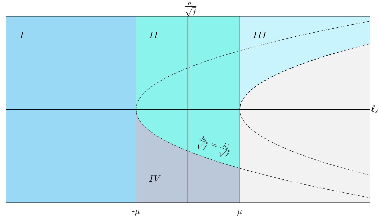
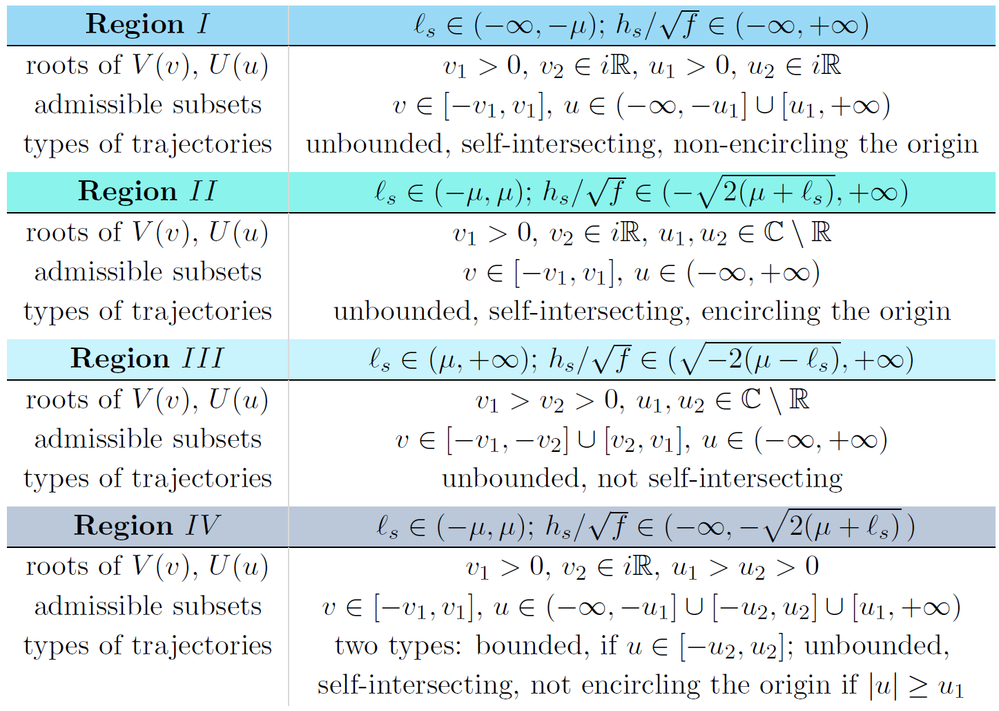
we have that the roots of $U(u)$ are $\pm {u}_1 , \pm {u}_2$, and those of $V(v)$ are $\pm {v}_1, \pm {v}_2$. As suggested in [Beletski, 1964], the problem can be studied in the $(\ell_s,h_s/\sqrt{f})$ plane, where four different regions can be identified characterised by different types of trajectories (see Figure 2). In the partotion of the $(\ell_s, h_s/\sqrt{f})$ plane which does not correspond to any of these regions, motion is not possible. The admissible subsets of the configuration space and the types of trajectories corresponding to the different regions are listed in the table in Figure 3.
In the admissible subsets of the configuration space zero velocity points exist only for some values $\ell_s, h_s$ of the integrals $\mathscr{L}_s,\mathscr{H}_s$ in regions $I$ and $IV$. Specifically, in the admissible subset corresponding to region $I$ we have the two points \((x,y) \in \{(\xi_1/2-\eta_1/2, \pm\sqrt{\xi_1\eta_1})\};\) instead, in the admissible subset corresponding to region $IV$ we have the four points \((x,y) \in \{(\xi_1/2-\eta_1/2, \pm\sqrt{\xi_1\eta_1}), (\xi_2/2-\eta_1/2, \pm\sqrt{\xi_2\eta_1})\}.\) In the subsets corresponding to regions $II$ and $III$ we do not find any zero velocity points.
Among the periodic orbits of Stark’s problem, there exists a family of unstable periodic orbits of brake type, which are orbits passing through zero velocity points. We denote the periodic orbit of brake type as \({\boldsymbol{x}}^* = {\boldsymbol{x}}^*(t;\ell_s)\): note that they parametrised by \(\ell_s \in (-\mu, \mu)\). Their energy is
then, the family exists for values $\ell_s, h_s$ corresponding to the boundary between regions $II$ and $IV$. In the Cartesian plane, \({\boldsymbol{x}}^*\) is a parabolic arc developing between the zero velocity points \((\xi^*/2-\eta_1^*/2, \pm\sqrt{\xi^*\eta_1^*})\), where \(\eta_1^*=\eta_1(h_s^*)\) and
\[\xi^* = -\frac{h_s^*}{f}.\]
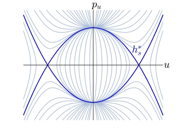
In the $(u,v)$ plane, \({\boldsymbol{x}}^*\) corresponds to two periodic orbit orbits of brake type, which have a constant value of the $u$-component, equal to \(\pm u^*\), and a constant value of \(p_u\), equal to $p_u^*$, with
\[p_u^* = 0 \qquad u^*=\sqrt{\xi^*}.\]On the other hand, the $v$-component is periodic. The orbits develop between the two zero velocity points given by \((u^*,\pm v_1^*)\), with \(v_1^*=\sqrt{\eta_1^*}\), in one case, and by \((-u^*, \pm v_1^*)\) in the other. These two orbits correspond to the two hyperbolic points appearing in the phase portrait of Stark’s problem in the $(u,p_u)$ plane, shown in Figure 4. The periodic orbit \({\boldsymbol{x}}^*\) is shown in Figure 5.
Sun-shadow dynamics
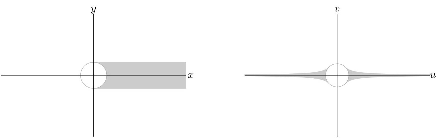
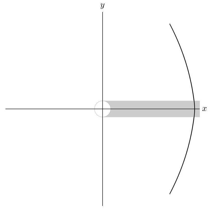
The Sun-shadow problem arises by patching Kepler’s dynamics in the shadow region and Stark’s dynamics in the remaining part of the configuration space. This implies that the the flow develops by alternating the two dynamics. In the Cartesian plane the Earth shadow region is defined as the set \(\{(x,y): \ x\geq0,\ -R\leq y \leq R\}\) with $R$ is the Earth radius. In the $(u,v)$ plane this region is doubled, i.e. it has two components as shown in Figure 6.
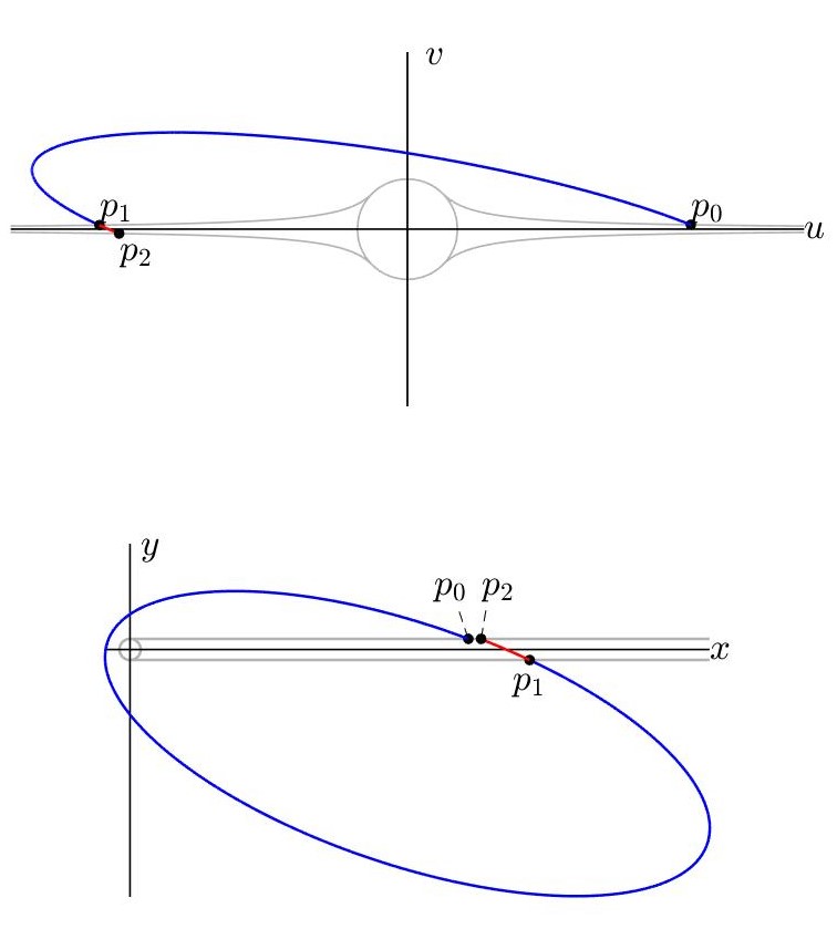
At the boundary of the shadow region, the subsets undergoes a leap in energy from $h_s$ to $h_k$ (or vice versa) and a leap from $\ell_s$ to $\ell_k$ (or vice versa). The variation of energy is equal to \(\pm f(\bar{u}^2-R^2/\bar{u}^2)/2\), with \(\bar{u}\) the value of $u$-component at the crossing point. Instead, $\ell_s-\ell_k= fR^2/2$. Each time the satellite returns in the out-of-shadow region, the \(\mathscr{L}_s\) assumes the same value it had before crossing the shadow, differently to the energy which changes unless the orbit is symmetric with respect to the $u$ axis. To understand this, uppose that at a time $\tau_0$ the body enters Stark’s regime at the point \(p_0 = (p_{u_{p_0}}, p_{v_{p_0}}, u_{p_0}, v_{p_0})\) (see Figure 7). Let \(h_{s_{p_0}}\) be the value of the energy and \(\ell_{s_{p_0}}\) the value of \(\mathscr{L}_s\). When the body returns to the shadow region through the point \(p_1\), we have a variation of the integrals given by
\[\begin{aligned} &h_{k_{p_1}} = h_{s_{p_0}} + \frac{f}{2}\biggl(u_{p_1}^2-\frac{R^2}{u_{p_1}^2}\biggr),\\ &\ell_{k_{p_1}} = \ell_{s_{p_0}} + \frac{f}{2} R^2\\ \end{aligned}\]with \(u_{p_1}\) the $u$ coordinate of \(p_1\). When the body goes back to Stark’s regime by passing through the point \(p_2 = (p_{u_{p_2}}, p_{v_{p_2}}, u_{p_2}, v_{p_2})\), we have similar variations equal to
\[\begin{aligned} & h_{s_{p_2}} = h_{k_{p_1}} - \frac{f}{2}\biggl(u_{p_2}^2-\frac{R^2}{u_{p_2}^2}\biggr),\\ &\ell_{s_{p_2}} = \ell_{k_{p_1}} - \frac{f}{2} R^2\\ \end{aligned}\]Thus, it holds
\[\begin{aligned} &h_{s_{p_2}} = h_{s_{p_0}} + \frac{f}{2}\biggl(1+\frac{R^2}{u_{p_1}^2 u_{p_2}^2}\biggr)\bigl(u_{p_1}^2-u_{p_2}^2\bigr),\\ &\ell_{s_{p_2}} = \ell_{s_{p_0}},\\ \end{aligned}\]with \(h_{s_{p_2}} = h_{s_{p_0}}\) only if \(u_{p_1}=u_{p_2}\).
There exists a family of periodic orbits of brake type, \(\widehat{\boldsymbol{x}}=\widehat{\boldsymbol{x}}(t;\ell_s)\), parametrised by $\ell_s$, which are close to the brake periodic orbits \(\boldsymbol{x}^*=\boldsymbol{x}^*(t;\ell_s)\) of Stark’s problem, described in the previous section. In the following, we summarize the proof of the existence of \(\widehat{\boldsymbol{x}}\).
Periodic Orbits of break type
Here we briefly outline the proof of the existence of the family of periodic orbits of brake type of the Sun-shadow dynamics. The main idea and the main passages of the demonstration are provided, without entering into the detail of the computations. For the complete proof, see [Cavallari, Gronchi, Baù, 2020].
To prove the existence of the family of periodic orbits of brake type, \(\widehat{\boldsymbol{x}}=\widehat{\boldsymbol{x}}(t;\ell_s)\), we consider values \(\ell_s \in (-\mu, \mu)\), for which the Stark’s periodic orbits \(\boldsymbol{x}^*\) exist. Successively, the interval \((-\mu,\mu)\) is restricted for reasons related to the proof. The idea of the proof is to search for an initial point \((x,y) = (x_0,0)\) in the shadow region with \(x_0>R\), such that the trajectory arrives to a zero velocity point in the out-of-shadow region, where we have Stark’s dynamics. The orbit is assumed symmetric with respect to the \(x\) axis, like \(\boldsymbol{x}^*\). Because of the symmetry, \(\widehat{\boldsymbol{x}}\) oscillates between two zero velocity points \((x_B,y_B)\) and \((x_B,-y_B)\). We search for an initial $x$-coordinate $x_0$ such that
\[x_0 > \xi^*/2,\]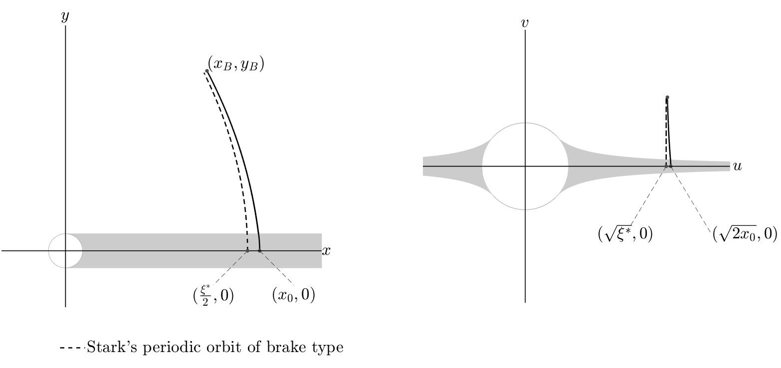
where \((\xi^*/2,0)\) belongs to \(\boldsymbol{x}^*\), see Figure 8. This condition is imposed since the pushing effect of the solar radiation pressure is lacking in the shadow region. The coordinate \(x_0\) must fulfil another condition: it must be such that at the exit point from the shadow region \((x_E,R)\), with \(x_E=x_E(x_0)\) we have
\[h_s < h_s^*,\]where \(h_s\) is the value of the energy in the out-of-shadow region and \(h_s^*\) is the energy of \(\boldsymbol{x}^*\) as well as the value of the energy at the boundary between Stark’s regions $II$ and $IV$. The last condition assures that the values of Stark’s first integrals in the out-of-shadow region are such that $(\ell_s, h_s/\sqrt{f})$ belongs to region $IV$; in this way, we can have zero velocity points in the admissible subset of the configuration space.
For the proof, the variables \(u,v\) are used. In the \((u,v)\) plane the initial point $(x_0,0)$ can correspond to both the points \((\pm \sqrt{2x_0},0)\) as well as the point \((\xi^*/2,0)\), which can correspond to \((\pm \sqrt{\xi^*},0)\). For symmetry reasons, we can focus on the \(\{u>0\}\) half-plane.
In Kepler’s regime the values of the integrals $\mathscr{H}_k$ and $\mathscr{L}_k$ are
\[h_k = -\frac{\mu+\ell_k}{2x_0}, \qquad \ell_k = \ell_ + \frac{f}{2}R^2\]and the initial state is of the type
\[(p_u,p_v,u,v)=(0,p_{v_0},\sqrt{2x_0},0), \qquad p_{v_0} = \sqrt{2(\mu-\ell_k)},\]because of the orbit symmetry with respect to the $x$ axis. Note that \(p_{v_0}\) has real values only by restricting the interval of \(\ell_s\) to \((-\mu,\mu-\frac{f}{2}R^2)\).
Assuming \(p_v>0\), the exit point from the shadow can be computed by solving
\[\left\{ \begin{aligned} &p_u^2 = 2h_k u^2 + 2(\mu + \ell_k)\\ &p_v^2 = 2h_k v^2 + 2(\mu - \ell_k)\\ &uv=R\\ &p_u p_v=2uv h_k, \\ \end{aligned} \right.\]It has coordinates \((u,v)=(\sqrt{\xi_E},R/\sqrt{\xi_E})\), with
\[\xi_E = x_0+x_T,\]where
\[x_T = x_T(x_0) = \sqrt{x_0^2 -a_k R^2}, \qquad a_k = \frac{\mu+\ell_k}{\mu-\ell_k}.\]In Cartesian coordinates, we have $x_E = \xi_E/2$.
The quantity $\xi_E$ has real values by further restricting the interval of $\ell_s$ to \([{\ell_s}^-,{\ell_s}^+]\), with
\[{\ell_s}^\pm = -\frac{5}{4}fR^2 \pm \sqrt{\mu^2+\frac{9}{16}f^2R^4-\frac{5}{2}fR^2\mu}.\]In the out-of-shadow region, the energy is given by
\[\mathsf{h}_s(x_0) = -\frac{\mu+\ell_k}{2x_0} -\frac{f}{2}\left(x_0+x_T\right) + \frac{fR^2}{2(x_0+x_T)}.\]We have that \(\mathsf{h}_s(x_0)\) is a strictly decreasing function of $x_0$ in the interval \((\xi^*/2,+\infty)\) and that there exists a value of $x_0$, \(x_0^*>\xi^*/2\), fulfilling \(\mathsf{h}_s(x_0^*)=h_s^*\). Thus, if \(x_0 \in (x_0^*,+\infty)\), it fulfils all the hypothesis previously made.
In this interval, it holds
\[2x_0>\xi_E > \xi_1 > \xi^* > \xi_2 > 0.\]Since \(\xi_E\) is the square of the $u$ coordinate at the exit point, we can conclude that in Stark’s regime the orbit belongs to unbounded subset of the possible configurations corresponding to region IV of Stark’s regime (see Figure 3).
Now, we introduce a further condition to be fulfilled so that the trajectory can reach a zero velocity point. We use the fictitious time $\tau$. The maps $u(\tau)$, $v(\tau)$ become stationary at $\tau=\tau_u, \tau_v$ respectively, with
\[\begin{aligned} \tau_u &= \int_{u_1}^{\sqrt{\xi_E}} \frac{du}{\sqrt{fu^4 + 2h_s u^2 + 2(\mu+\ell_s)}},\\ \tau_v &= \int_{\frac{R}{\sqrt{\xi_E}}}^{v_1} \frac{dv}{\sqrt{- fv^4 + 2h_s v^2 + 2(\mu-\ell_s)}}.\\ \end{aligned}\]So, we need to search for $x_0$ such that
\[\tau_u = \tau_v.\]From now on, it is more convenient to use \(h_s \in J =(-\infty, h_s^*)\) as independent variable, in place of \(x_0 \in (x_0^*,+\infty)\). We have that $\tau_u$ is a strictly increasing function of $h_s$ and
\[\lim_{h_s \to h_s^*} \tau_u = +\infty,\]while $\tau_v$ is such that
\[\limsup_{h_s \to h_s^*} \tau_v < +\infty.\]Hence, to show that equation $\tau_u = \tau_v$ has solution, we only need to search for a value of the energy $h_s \in J$ such that \(\tau_u(h_s) < \tau_v(h_s).\)
This value is found by means of estimates of $\tau_u$ and $\tau_v$. Indeed, there exist \(\bar{h}_s\in J\) and two functions $\tilde{\tau}_u(h_s), \tilde{\tau}_v(h_s)$ fulfilling
\[\tau_v(\bar{h}_s) > \tilde{\tau}_v(\bar{h}_s) = \tilde{\tau}_u(\bar{h}_s) > \tau_u(\bar{h}_s),\]where
\[\tilde{\tau}_u(h_s) = \frac{1}{\sqrt{f}} \frac{\left(1+\frac{1}{\xi^*}\sqrt{\frac{2(\mu-\ell_s)}{f}}\right)^{1/2}}{\left(\xi_1+\sqrt{\frac{2(\mu-\ell_s)}{f}}\right)^{1/2}} \frac{1}{\sqrt{ 1 + \frac{\xi_1-\xi_2}{C_2}}-1 },\\\]with
\[C_2 = R\sqrt{\frac{1-C+2 a_k}{1+C}}, \qquad C = \sqrt{1 - 4 a_k\frac{R^2}{\xi^{*^2}}},\]and
\[\tilde{\tau}_v (h_s) = \frac{1}{\sqrt{2f}\left(\xi_1+\sqrt{\frac{2(\mu-\ell_s)}{f}}\right)^{1/2}}\arcsin\sqrt{1-\frac{R^2}{\xi^*\eta_1^*}}, \qquad \eta_1^* = \eta_1(h_s^*) = -\xi^* + 2\sqrt{\mu/f}.\]Setting
\[K_1 = \sqrt{2} \left(1+\frac{1}{\xi^*}\sqrt{\frac{2(\mu-\ell_s)}{f}}\right)^{1/2}, \qquad K_2 = \arcsin\sqrt{1-\frac{R^2}{\xi^*\eta_1^*}},\]the energy value \(\bar{h}_s\) is given by
\[\bar{h}_s =-f \left( \xi^{*^2}+\frac{C_2^2}{4}\frac{K_1^2}{K_2^2}\left(2+\frac{K_1}{K_2}\right)^2\right)^{1/2}.\]This result allows to conclude that the family of brake periodic orbits $\widehat{\boldsymbol{x}}(t;\ell_s)$ exists. In Figure 9 \(\widehat{\boldsymbol{x}}\) is shown.
Sun-shadow map
To obtain a deeper insight on the Sun-shadow dynamics, it is useful to employ a Poincaré map. In case of autonomous Hamiltonian systems, a Poincaré map is typically defined by fixing the value of the Hamiltonian in addition to a specific section in the configuration space. This is not possible for the Sun-shadow problem; indeed, the Hamiltonian is not a first integral. However, it is possible to fix the value of \(\mathscr{L}_s\): even though \(\mathscr{L}_s\) is not a constant of motion as well, it always has the same value in the out-of-shadow region, where we have Stark’s dynamics. As section we selected the upper boundary of the shadow region in the Cartesian plane and we considered trajectories leaving the boundary with $p_y>0$. Despite the section was conceived in the $(x,y)$-plane, the map is defined using the variables $p_u,p_v,u,v$:
\[\begin{aligned} \mathfrak{S}: \mathcal{D} \subset\mathbb{R}^2 &\to \mathbb{R}^2,\\ (u,p_u) &\mapsto (u',p'_u),\\ \end{aligned}\]where $(u,p_u),(u’,p’_u)$ belong to the section $\Sigma$
\[\Sigma = \{(p_u,p_v,u,v): \ |u|\geq \sqrt{R},\ uv = R, \ up_v > \max(0,-p_uv), \ \mathscr{L}_s = \ell_s\}.\]In the following, the map is called Sun-shadow map. In the definition, condition $up_v>-p_uv$ corresponds to $p_y>0$. Moreover, condition $up_v>0$ is added so that every point $(u,p_u)\in\Sigma$ corresponds to only one trajectory; without this condition, there would be points $(u,p_u)\in\Sigma$ for which $p_y>0$ for both $p_v>0$ and $p_v<0$.
The domain \(\mathcal{D}\) does not coincide with \(\mathbb{R}^2\), since it does not include the three following subsets: \(\mathcal{D}_{\infty} \subset\mathbb{R}^2\), made by the points corresponding to trajectories which go to inifinity before going back to \(\Sigma\); \(\mathcal{D}_{C} \subset\mathbb{R}^2\), made by the points corresponding to trajectories which collide with the Earth before going back to \(\Sigma\); \(\mathcal{D}_{F} \subset\mathbb{R}^2\), made by the points for which either the motion is not possible or the map is not defined. Specifically, \(\mathcal{D}_{F}\) includes all the points $(u,p_u)$ with
\[p^2_u \leq 2(\mu+\ell_s) + fR^2 + (f-2(\mu-\ell_s)/R^2)u^4.\]
that are the points for which \(p_v^2\leq0\). Moreover, all the points in the second and fourth quadrant of the $(u,p_u)$ plane belong to the subset \(\mathcal{D}_{F}\) if $\ell_s > \mu - \frac{fR^2}{2}$, since they do not fulfil the condition \(up_v > \max(0,-p_uv)\); if $\ell_s \leq \mu - \frac{fR^2}{2}$, the latter condition is not fulfilled only by the points of the second and fourth quadrant with
\[u^4\leq\frac{2(\mu+\ell_s)+fR^2}{2(\mu-\ell_S)-fR^2}R^2.\]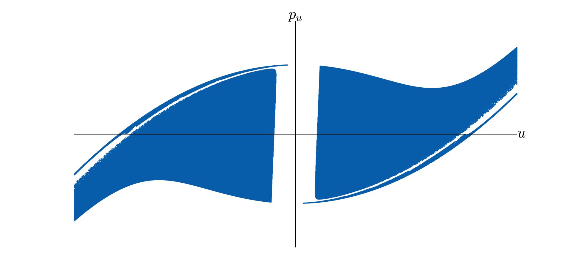
In Figure 10, for a specific choice of $\ell_s$ and $f$, a portion of the domain \(\mathcal{D}\) is drawn in white on the $(u,p_u)$ plane. The light grey region corresponds to the set $\mathcal{D}_{F}$. The other two coloured areas contain portions of the sets \(\mathcal{D}_{\infty}\) (darker blue) and \(\mathcal{D}_{C}\) (light blue). Figure 11 shows a portion of the image of \(\mathcal{D}\) under the map $\mathfrak{S}$. It is possible to observe that the image of the map contains points which belong to \(\mathcal{D}_{\infty}\) or \(\mathcal{D}_{C}\): for those points, the map can not be further iterated.
The map $\mathfrak{S}$ is differentiable in its definition domain \(\mathcal{D}\), but it is not area preserving. Moreover, given $\ell_s \in [\ell_s^{-},\ell_s{+}]$, the periodic orbit of brake type \(\widehat{\boldsymbol{x}}(t;\ell_s)\) gives rise to two fixed points $\widehat{\boldsymbol{\upsilon}}_{1,2}$ of the Sun-shadow map, i.e.
\[\widehat{\boldsymbol{\upsilon}}_1= (\sqrt{\xi_E},-p_{u_E}), \qquad \widehat{\boldsymbol{\upsilon}}_2= (-\sqrt{\xi_E},p_{u_E}),\]with
\[p_{u_E}^2 = 2\widehat{h}_s\xi_{\tiny E}+2(\mu+\ell_s)+f\xi_{\tiny E}^2,\qquad p_{u_E}>0,\]where $\widehat{h}_s$ is the energy of \(\widehat{\boldsymbol{x}}\) in the out-of-shadow region. The point $\widehat{\boldsymbol{\upsilon}}_1$ lies in the region included into the small rectangle in Figure 10. By numerical computation, it results that the Jacobian matrix of the map at \(\widehat{\boldsymbol{\upsilon}}_{j}\), \(j=1,2\) has two real eigenvalues $\lambda^j_1,\lambda^j_2$ with
\[0<\lambda_1^{j}<1<\lambda_2^{j}.\]This implies that the two fixed points are hyperbolic and that the periodic orbit of brake type is unstable. In the following, we summarize the techinique used for the computation of their invariant manifolds.
Invariant Manifold
Here, we summarize the numerical technique used to compute the invariant manifolds of \(\widehat{\boldsymbol{\upsilon}}_1\); the same procedure can be applied also for \(\widehat{\boldsymbol{\upsilon}}_2\). The method used is inspired by [Hobson, 1993] and it is suitable to two-dimensional maps which have saddle-type fixed points and a Jacobian matrix evaluated at these points with two real eigenvalues $\lambda_1,\lambda_2$ such that $0<\lambda_1<1<\lambda_2$: the Sun-shadow $\mathfrak{S}$ fulfils both these conditions. Let us suppose we want to compute one branch $B$ of the unstable manifold. The method consists in dividing the branch of the manifold into a sequence of connected subset $V$, which are called primary segments. Once determined an initial primary $V_0$ in a small neighbourhood of \(\widehat{\boldsymbol{\upsilon}}_1\), all the other primaries can be computed by iterating the map $m$ times:
\[V_{i+1} = \mathfrak{S}(V_{i}), \qquad i = 0,\ldots,m-1.\]Then, the branch will be given by
\[B = \bigcup_i V_i.\]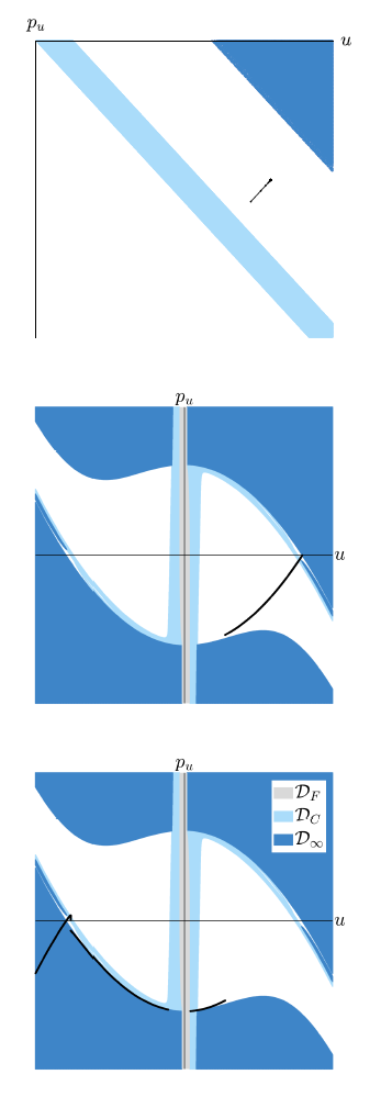
The initial primary can be approximated by a small segment very close to the fixed point along an unstable eigenvector of the Jacobian \(D\mathfrak{S}(\widehat{\boldsymbol{\upsilon}}_1)\). It is then corrected by using the technique described in [Lega, Guzzo, 2016], based on the Modified Fast Lyapunov Indicators (MFLI).
The same procedure can be applied to construct the branches of the stable manifold using the inverse map $\mathfrak{S}^{-1}$.
After few iterations, portions of the primaries are lost because the corresponding trajectories do not return to section $\Sigma$; thus, the primaries lose their nature of connected sets. To understand the phenomenon, consider Figure 12, which shows the first steps in the computation of a branch of the unstable manifold. In the background, there is a portion of the domain of the map. The initial primary \(V_0\) (top) is iterated once under the map. Its image $V_1$ (middle) intersects the forbidden region \(\mathcal{D}_{C}\). The consequence is that at the second iteration, the primary $V_2$ has three different components (bottom). Note that $V_2$ intersects the forbidden regions \(\mathcal{D}_{C}\), \(\mathcal{D}_{\infty}\). Thus, the number of components will increase at successive iterations. We can conclude that the invariant manifold is made by several connected componens.
Global picture of the Sun-shadow map
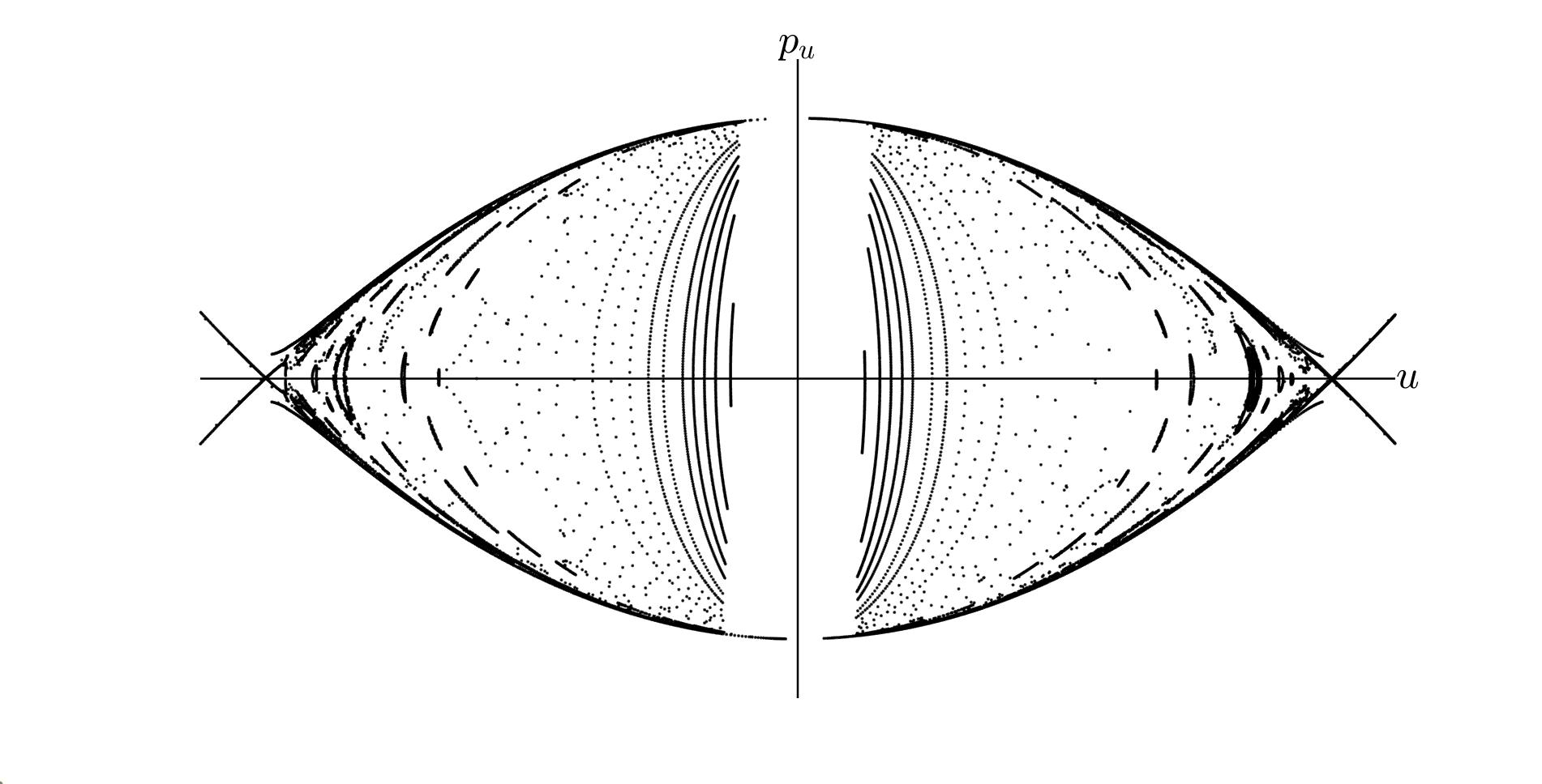
Figure 13 shows a global picture of the Sun-shadow map. There is evidence of regular and chaotic behaviour, with the presence of several islands. We numerically verified that some of the islands surround periodic points. In the central region of the global picture, a regular structure seems to exist, similar to the one of the phase portrait in Figure 4. On the other hand, a chaotic behaviour seems to appear in a neighbourhood of \(\widehat{\boldsymbol{\upsilon}}_1\), along the stable and unstable branches of its invariant manifold.