Close encounters
Planetary close encounters can drastically modify the heliocentric orbits of small bodies, such as asteroids or comets (see [Battin, 1999]). The phenomenon is of interest for several reasons. For example, as explained in [Greenberg et al., 1988], close encounters should be taken into account to study the processes of planetary accretion. The problem is significant also in the context of the orbit determination; indeed, the identity of small bodies can become uncertain as a consequence of a close encounter, because of the drastic change of their heliocentric mean orbital elements. Moreover, the problem of close encounters is important in the framework of planetary defence and impact monitoring.
Beyond the application of a three-body model (which is not integrable), two methods have been used so far to study the dynamics of planetary close encounters: Öpik’s method and the patched-conics method. In both the methods, the trajectory between encounters is assumed as an unperturbed heliocentric Keplerian orbit; during the encounter, all the forces acting on the small body are neglected, except for the gravity of the planet. The difference between the methods lies in the approximations employed to model the encounter, which will be described below.
To justify the application of both Öpik’s method and the patched-conics method, consider the equations of motion of a small body, expressed in terms of both heliocentric and planetocentric coordinates:
\[\ddot{\boldsymbol{r}} = -\frac{GM_{\odot}\boldsymbol{r}}{\vert\boldsymbol{r}\vert^3} - \frac{Gm_{p}}{\vert\boldsymbol{d}\vert^3}{\boldsymbol{d}},\] \[\ddot{\boldsymbol{d}} = - \frac{Gm_{p}}{d^3}{\boldsymbol{d}} -\frac{GM_{\odot}\boldsymbol{r}}{\vert\boldsymbol{r}\vert^3} -\frac{GM_{\odot}}{\vert\boldsymbol{r}\vert^3}\Big(1-\frac{\vert\boldsymbol{r}\vert}{\vert\boldsymbol{r_p}\vert}\Big)\boldsymbol{r}_p;\]$\boldsymbol{r}$ and $\boldsymbol{d}$ are the heliocentric and planetocentric position vectors of the small body, respectively; $\boldsymbol{r_p}$ is the heliocentric position vector of the planet; $G$ is Newton’s gravitational constant and $M_{\odot}$ and $m_p$ are the Sun and the planet’s masses. The small body is approximated as a massless particles. Since $M_{\odot}»m_p$, if the body is far from the planet ($\vert\boldsymbol{d}\vert$ is large) the term $\frac{Gm_{p}}{\vert\boldsymbol{d}\vert^3}{\boldsymbol{d}}$ can be neglected in the first equation. Thus, we obtain the equation of motion typical of Kepler’s problem with the Sun as center of mass:
\[\ddot{\boldsymbol{r}} = -\frac{GM_{\odot}\boldsymbol{r}}{\vert\boldsymbol{r}\vert^3}.\]On the contrary, this approximation is not suitable if the body is close to the planet, i.e. if $\vert\boldsymbol{d}\vert$ is close to zero. In this case, it’s the term $\frac{GM_{\odot}\boldsymbol{r}}{\vert\boldsymbol{r}\vert^3}$ to become negligible in comparison to $\frac{Gm_{p}}{\vert\boldsymbol{d}\vert^3}{\boldsymbol{d}}$. Moreover, if $\vert\boldsymbol{d}\vert\sim 0$, we also have that $\vert\boldsymbol{r}\vert\sim \vert\boldsymbol{r}_p\vert$. Thus we can neglect the second and the third terms in the planetocentric equation of motions, obtaining the equation of motion typical of Kepler’s problem with the planet as center of mass:
\[\ddot{\boldsymbol{d}} = - \frac{Gm_{p}}{d^3}{\boldsymbol{d}}.\]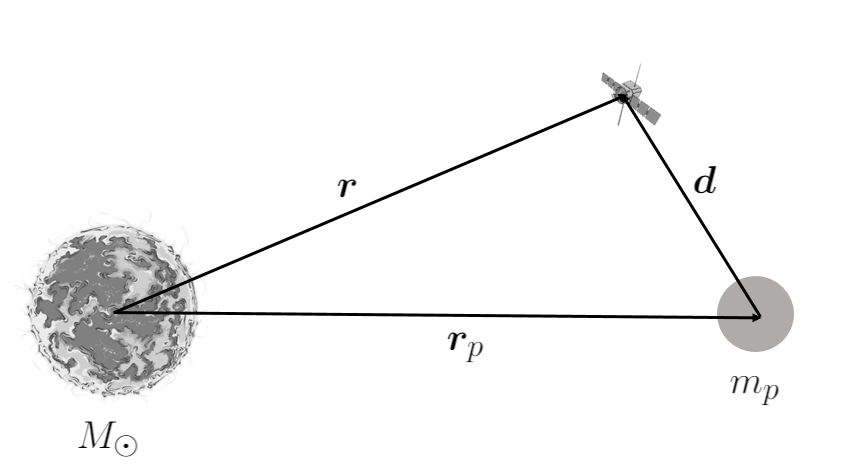
Currently, Öpiks’s model is extensively applied to study close-encounters. Conversely, the patched-conics method is rarely used to study close encounters.
In the following, we summarize Öpik’s model. Then, we discuss the patched-conics method, and show the advantage it has in the framework of resonant returns.
Table of Contents
Öpik method
The original Öpik’s method is thought to deal with planetary close encounters affecting small bodies whose heliocentric trajectory intersect the planet’s orbit. The encounter is modelled as an instantaneous two-body scattering between the body and planet, which takes place at the intersection of their orbits (see [Carusi & Valsecchi, 1990]). As explained in [Greenberg et al., 1988], in order to apply the method the argument of the perihelion and the initial mean anomaly of the body are adjusted to force the planet and the body to reach the same position at the same time. The consequence of the encounter is an instantaneous variation of the heliocentric velocity of the body.
Öpik’s theory was extended in [Valsecchi et al., 2003] and [Valsecchi, 2006] to deal with orbits which do not intersect the planet’s one. The approximations employed to model the encounter are based on the hypothesis that the body’s trajectory at the encounter can be considered a Keplerian hyperbolic orbit which has the planet as center of mass (as in the patched-conics approximation). When the body gets sufficiently close to the planet, its motion is approximated as uniform and linear along the incoming asymptote of the hyperbola with a velocity equal to the incoming hyperbolic excess velocity $\boldsymbol{U}$. At an instant $t_0$, the body crosses the b-plane i.e. the plane passing through the planet’s center and orthogonal to $\boldsymbol{U}$. At $t_0$, the uniform and linear motion stops and an instantaneous transition from the incoming to the outgoing asymptotes of the hyperbola is performed. Finally, a uniform and linear motion along the outgoing asymptote with velocity equal to outgoing hyperbolic excess velocity leads the body to its new heliocentric Keplerian orbit.
In [Valsecchi et al., 2003], Valsecchi et al. introduced a set of non-canonical coordinates suitable to analyse close encounters. These coordinates are $U,\theta,\phi,\xi_V,\zeta_V,t_0$: $U=\vert\boldsymbol{U}\vert$; $\theta$ and $\phi$ are the angles defining the orientation of $\boldsymbol{U}$ in a Cartesian planetocentric reference frame; $\xi_V$ and $\zeta_V$ are the coordinates defined on the b-plane such that $\sqrt{\xi_V^2+\zeta_V^2}=b$, with $b$ the impact parameter equal to the distance between the planet’s center and the hyperbola’s asymptotes; $t_0$ is the time at which the asteroid crosses the b-plane.
Examples of application of the extended Öpik’s method for the problem of planetary close encounter are given in [Milani et al., 1999], [Milani et al., 2005], [Valsecchi et al., 2018], [Valsecchi et al., 2019], [Farnocchia et al., 2019]; the method has also been used to study spacecrafts swing-by in [Valsecchi et al., 2015].
Patched-Conics Method
Close encounters can be studied by means of the patched-conics approximation. The asteroid (or the comet) is modelled as a massless particle, traveling along an unperturbed heliocentric Keplerian elliptic orbit before and after the encounter. The encounter occurs inside the sphere of influence of the planet, where the trajectory of the asteroid is considered as an unperturbed planetocentric Keplerian hyperbolic orbit. Assuming that the orbit of the planet is circular (which is a reasonable approximation for a large number of planets in the Solar system), the sphere of influence consists in a spherical region of the configuration space surrounding the planet and centered at the planet’s center.
The reason why the application of the patched-conics approximatation in the framework of close encounters is still uncommon is related to the ambiguity existing in the definition of the planet’s sphere of influence. Classicaly, the sphere of influence employed is either Hill’s sphere or Laplace’s sphere (see [Cheboratev, 1964]). Hill’s sphere and Laplace’s sphere have radius equal to
\[R_{H}=\Big(\frac{m_p}{3M_{\odot}}\Big)^{\frac{1}{3}}, \quad R_{L}=\Big(\frac{m_p}{M_{\odot}}\Big)^{\frac{2}{5}},\]respectively.
$R_{H}$ approximates the distance between the Earth’s center and the Sun-Earth’s Lagrange point $L_1$. Indeed, as shown in [Szebehely, 1967]) the distance $\xi_1$ of the Earth from $L_1$ can be determined as a power series in the quantity $\nu=R_{H}$:
\[\xi_1 = \nu-\frac{1}{3}\nu^2 -\frac{1}{9}\nu^4 +{O}(\nu^5).\]If we truncate this series at the first order in $\nu$, $\xi_1$ is equal to $R_H$.
$R_{L}$ is the estimated radius of a spherical region around the planet: inside this region, the perturbing effect of the Sun on the body’s planetocentric orbit is lower than the perturbing effect of the planet on the body’s heliocentric orbit. The derivation of $R_{L}$ is shown in [Curtis, 2010]) and it is based on a comparison between the perturbing accelerations of the heliocentric and planetocentric orbits of the body.
In [Cheboratev, 1964]), Cheboratev introduced a further definition of sphere of influence, which he called “Gravitational sphere of the planet” and which is called “Cheboratev’s sphere” in [Souami et al., 2020]. Using Cheboratev’s words, it is “the region of space within which the attraction of the planet is greater than solar attraction”. The radius of Cheboratev’s sphere is
\[R_{C}=\Big(\frac{m_p}{M_{\odot}}\Big)^{\frac{1}{2}}.\]As shown in [Souami et al., 2020], it holds $R_{C}<R_{L}<R_{H}$.
The definitions of sphere of influence introduced have a similarity: all of them depend only on the ratio between the masses of the planet and the Sun and are independent of the dynamics of the small body. However, in [Wetherill & Cox, 1984] (where Laplace’s sphere is employed) it emerges that the two-body approximation can fail depending on the relative velocity of the asteroid with respect to the planet. Also in [Araujo et al., 2008] it is shown through a numerical study that the radius of the sphere of influence should depend on the relative velocity.
Despite of the problem concerning the definition of the sphere of influence, the patched-conics approximation presents an advantage in the framework of resonant returns. After a close encounter, the body can enter a heliocentric orbit whose orbital period is commensurable to the orbital period $T_{p}$ of the planet:
\[\frac{T'}{T_{p}}=\frac{k_{p}}{k'}, \quad k_{p},k'\in\mathbb{Z}\setminus\{0\}\]where
\[T' = 2\pi\sqrt{\frac{a'^3}{GM_{\odot}}};\]$a’$ is the post-encounter heliocentric semi-major axis of the asteroid. In this case, after an amount of time equal to $k’T’$ the body and the planet return to the same relative position of the previous post-encounter. Thus, after a time slightly smaller than $k’T’$, we expect a new close-encounter: the asteroid will enter again the sphere of influence and a so-called resonant return will occur. Through the patched-conics method, it is possible to treat resonant returns by means of canonical transformations, as shown in the following. More details about the results below can be found in [Grassi, Cavallari, Gronchi, Baù, in preparation].
Resonant encounter as a canonical transformation
We show that it is possible to consider a sequence of canonical transformations from the entrance of the sphere of influence at the first encounter to the entrance of the sphere of influence at the second encounter. Let us set:
- $(\boldsymbol{p}_H^{(0)},\boldsymbol{x}_H^{(0)})$ the heliocentric Cartesian coordinates of the body before the first encounter;
- $(\boldsymbol{p}_P^{(0)},\boldsymbol{x}_P^{(0)})$ the planetocentric Cartesian coordinates of the body at the entrance of the sphere of influence at the first encounter;
- $(\boldsymbol{p}_P^{(1)},\boldsymbol{x}_P^{(1)})$ the planetocentric Cartesian coordinates of the body at the exit from the sphere of influence at the first encounter;
- $(\boldsymbol{p}_H^{(1)},\boldsymbol{x}_H^{(1)})$ the new heliocentric Cartesian coordinates at the exit from the sphere of influence at the first encounter;
- $(\boldsymbol{p}_H^{(2)},\boldsymbol{x}_H^{(2)})$ the heliocentric Cartesian coordinates before the second encounter;
- $(\boldsymbol{p}_P^{(2)},\boldsymbol{x}_P^{(2)})$ the planetocentric Cartesian coordinates of the body at the entrance of the sphere of influence at the second encounter.
The transformation $(\boldsymbol{p}_{H}^{(0)},\boldsymbol{x}_H^{(0)})\mapsto (\boldsymbol{p}_P^{(0)},\boldsymbol{x}_P^{(0)})$ is given by
\[\boldsymbol{x}_P^{(0)} = \boldsymbol{x}_H ^{(0)} - \boldsymbol{r}_p(t_0), \quad \boldsymbol{p}_P^{(0)} = \boldsymbol{p}_H^{(0)} - \dot{\boldsymbol{r}}_p(t_0)\]with $(\boldsymbol{r}_p(t_0),\dot{\boldsymbol{r}_p}(t_0)$ the heliocentric Cartesian coordinates of the planet. The transformation is simply a translation and therefore it is canonical.
Inside the sphere of influece, the dynamics is Keplerian and planetocentric with Hamiltonian function \({H}_P(\boldsymbol{p}_P,\boldsymbol{x}_P) = \frac{\vert\boldsymbol{p}_P\vert^2}{2}-\frac{Gm_p}{\vert\boldsymbol{x}_P\vert}.\)
The coordinates $(\boldsymbol{p}_P^{(1)},\boldsymbol{x}_P^{(1)})$ at the exit from the sphere of influence are given by the hyperbolic motion of the body. The exit and the entrance points are symmetric with respect to the line of apsis of the hyperbolic orbit. The time $\Delta t = t_1-t_0$ it takes the body to go from the entrance point to the exit point depends on the initial conditions $(\boldsymbol{p}_P^{(0)},\boldsymbol{x}_P^{(0)})$. From the Hamiltonian theory, we know that the map given by the Hamiltonian flow with fixed end-time is canonical. To obtain a fixed-time transformation, we perform a time rescaling. We introduce a fictitious time $\tau$ defined through the relation
\[\sigma(\boldsymbol{p}_P^{(0)},\boldsymbol{x}_P^{(0)}) d\tau=dt\]where \(\sigma(\boldsymbol{p}_P^{(0)},\boldsymbol{x}_P^{(0)})\) is a function of the initial conditions, independent of time. The fictitious time \(\tau_{\small{\mbox{hyp}}}\) from the entrance to the exit of the sphere of influence is equal to
\[\tau_{\small{\mbox{hyp}}} = \int_{t_0}^{t_1} \frac{1}{\sigma(\boldsymbol{p}_P^{(0)},\boldsymbol{x}_P^{(0)}) }dt = \frac{t_1-t_0}{\sigma(\boldsymbol{p}_P^{(0)},\boldsymbol{x}_P^{(0)}) },\]with $t_1=t_1(\boldsymbol{p}_P^{(0)},\boldsymbol{x}_P^{(0)})$.
We choose $\tau_{\small{\mbox{hyp}}}=1$ so that \(\sigma(\boldsymbol{p}_P^{(0)},\boldsymbol{x}_P^{(0)})= t_1(\boldsymbol{p}_P^{(0)},\boldsymbol{x}_P^{(0)})-t_0\). Now, we can introduce the new Hamiltonian
\[K_P(\boldsymbol{p}_{P},\boldsymbol{x}_P) = \sigma(\boldsymbol{p}_P,\boldsymbol{x}_P) \Big( H_P(\boldsymbol{p}_P,\boldsymbol{x}_P) - E_{\small{\mbox{hyp}}} \Big),\]where \(E_{\small{\mbox{hyp}}}\) is a constant.
The map $\Phi_{K_P}^{0,\tau_{\tiny{\mbox{hyp}}}}$ of the Hamiltonian flow with Hamilton’s function $K_P$ gives a canonical transformation since the propagation time $\tau_{\small{\mbox{hyp}}}$ is constant for all initial conditions. If we restrict to the energy level set \(H_P(\boldsymbol{p}_P,\boldsymbol{x}_P)=E_{\small{\mbox{hyp}}}\), the trajectories defined by the Hamiltonian flows \(\Phi_{K_P}^{0,\tau}\) and $\Phi_{H_P}^{t_0,t}$ coincide.
The post-encounter heliocentric coordinates $(\boldsymbol{p}_H^{(1)},\boldsymbol{x}_H^{(1)})$ are
\[\boldsymbol{x}_H^{(1)} = \boldsymbol{x}_P ^{(1)}+\boldsymbol{r}_p(t_1), \quad \boldsymbol{p}_H^{(1)} = \boldsymbol{p}_P^{(1)} + \dot{\boldsymbol{r}}_p(t_1).\]After the encounter, the Sun-body Keplerian dynamics is defined by the Hamiltonian ${H}_H$, equal to
\[{H}_H = \frac{\vert\boldsymbol{p}_H\vert^2}{2}-\frac{GM_{\odot}}{\vert\boldsymbol{x}_H\vert};\]If the new semi-major axis $a’$ fulfils relation
\[2\pi\sqrt{\frac{a'^3}{M_{\odot}}}k'=k_{p}T_p, \quad k_{p},k'\in\mathbb{Z}\setminus\{0\}\]there will be a second close encounter between the body and the planet. Let $\Delta t = t_2-t_1$ be the time it takes the body to go from the exit of the sphere of influence at the first encounter to the entrance of the sphere of influence at the second encounter. As in the case of the planetocentric hyperbolic motion inside the sphere of influence, $t_2$ depends on \((\boldsymbol{p}_H^{(1)},\boldsymbol{x}_H^{(1)})\). In order to have a canonical transformation from the first to the second encounter, we consider a rescaling of the time as done before. Following the same steps previously performed, we get a Hamiltonian \(K_H\) that describes the heliocentric elliptic motion when restricted to the energy level \(H_H(\boldsymbol{p}_H,\boldsymbol{x}_H)=E_{\small{\mbox{ell}}}\), with \(E_{\small{\mbox{ell}}}=-\frac{GM_{\odot}}{2a'}\). It is possible to observe that fixing $E_{\small{\mbox{ell}}}$ (i.e. \(a'\)) implies fixing the resonance condition \(k_p/k'\).
Once obtained \((\boldsymbol{p}_H^{(2)},\boldsymbol{x}_H^{(2)})\), the new coordinates \((\boldsymbol{p}_P^{(2)},\boldsymbol{x}_P^{(2)})\) are
\[\boldsymbol{x}_P^{(2)} = \boldsymbol{x}_H ^{(2)} - \boldsymbol{r}_p(t_2), \quad \boldsymbol{p}_P^{(2)} = \boldsymbol{p}_H^{(2)} - \dot{\boldsymbol{r}}_p(t_2).\]We constructed a canonical transformation which corresponds to the map of the resonant return when we select initial conditions belonging to a subset of the phase space defined by the energy constraints previously described.
Canonical coordinates on the b-plane
Following the work [Tommei, 2006], we show that there exists a set of canonical variables which are related to Valsecchi’s b-plane coordinates used in the extended Öpik’s theory. We introduce the coordinates $(\xi, \eta, \zeta, P_\xi, P_\eta, P_\zeta)$ such that $P_{\zeta}=U$ and $\xi$ and $\zeta$ fulfil the same relation existing between $\xi_V$ and $\eta_V$, i.e.
\[\xi^2+\zeta^2=b^2.\]In particular, $\xi$ and $\zeta$ are defined on a plane which is parallel to the b-plane.
Let us consider the hyperbolic Delaunay variables: $L,G,H,\ell,g,h$. We recall
\[\begin{aligned} & L =-\sqrt{\mu a_P} & &\ell=e_P\sinh F_P-F_P\\ & G =\sqrt{\mu a_P(e_P^2-1)} & &g=\omega\\ & \Theta =\sqrt{\mu a_P(e_P^2-1)}\cos(i_P) & &h=\Omega \end{aligned}\]where $\mu=Gm_{p}$ and $(a_P,e_P,i_P,\Omega_P,\omega_P,F_P)$ are the Keplerian elements of the planetocentric orbit ($F_P$ is the hyperbolic eccentric anomaly). We have that the magnitude of the incoming hyperbolic excess velocity $U$ and of the impact parameter $b$ are
\[U=\sqrt\frac{\mu}{a_P}=-\frac{\mu}{L}\, \quad b=a_P\sqrt{e_P^2-1}=-\frac{L}{\mu}G\ .\]As in [Tommei, 2006], we look for canonical coordinates $(\xi, \eta, \zeta, P_\xi, P_\eta, P_\zeta)$ such that
- i) only $\eta$ depends on the mean anomaly $\ell$,
- ii) $\xi^2+\zeta^2=b^2$.
Moreover, as in [Tommei, 2006], taking a rectangular coordinate system $(\xi,\zeta)$ we express $\xi$ and $\zeta$ as
\[\xi=b\cos\psi, \quad \zeta=b\sin\psi,\]for some angle $\psi=\psi(L,G,H,g,h)$.
Using the definition of $U$, it holds
\[\begin{aligned} &\{\xi,\zeta\}=\frac{\partial\xi}{\partial G}\frac{\partial\zeta}{\partial g}-\frac{\partial\xi}{\partial g}\frac{\partial\zeta}{\partial G}+\frac{\partial\xi}{\partial H}\frac{\partial\zeta}{\partial h}-\frac{\partial\xi}{\partial h}\frac{\partial\zeta}{\partial H}=\\ &\quad=\Biggl(-\frac{L}{\mu}\cos\psi+\frac{LG}{\mu}\sin\psi\frac{\partial\psi}{\partial G}\Biggr)\Biggl(-\frac{LG}{\mu}\cos\psi\frac{\partial\psi}{\partial g}\Biggr)-\\&\quad-\Biggl(\frac{LG}{\mu}\sin\psi\frac{\partial\psi}{\partial g}\Biggr)\Biggl(-\frac{L}{\mu}\sin\psi-\frac{LG}{\mu}\cos\psi\frac{\partial\psi}{\partial G}\Biggr)+\\ &\quad+\Biggl(\frac{LG}{\mu}\sin\psi\frac{\partial\psi}{\partial H}\Biggr)\Biggl(-\frac{LG}{\mu}\cos\psi\frac{\partial\psi}{\partial h}\Biggr)-\Biggl(\frac{LG}{\mu}\sin\psi\frac{\partial\psi}{\partial h}\Biggr)\Biggl(-\frac{LG}{\mu}\cos\psi\frac{\partial\psi}{\partial H}\Biggr)\\ &\quad=\frac{L^2G}{\mu^2}\frac{\partial\psi}{\partial g}\, . \end{aligned}\]Then, to have ${\xi,\zeta}=0$, $\psi$ can not depend on $g$. We choose $\psi=h$.
Our goal is to determine $\eta$ such that its conjugated momentum $P_{\eta}$ is equal to $U$. We extend the relations
\[\xi=-\frac{LG}{\mu}\cos h,\quad\zeta=-\frac{LG}{\mu}\sin h,\quad P_\eta=U=-\frac{\mu}{L} .\]to a canonical transformation
\[(L,G,H,\ell,g,h) \mapsto (P_\xi, P_\eta, P_\zeta,\xi,\eta,\zeta)\]by means of the generating function
\[S = S(\ell,g,H,\xi,\zeta,P_\eta) = -\frac{\mu}{P_\eta}\ell+gP_\eta\sqrt{\xi^2+\zeta^2}-H\arctan\biggl(\frac{\zeta}{\xi}\biggr)\,.\]Using relations
\[L=-\frac{\mu}{P_\eta}\, ,\quad G=P_\eta\sqrt{\xi^2+\zeta^2}\, ,\quad h=\arctan\biggl({\frac{\zeta}{\xi}}\biggr)\, ,\]we get
\[\begin{aligned} P_\xi=-\frac{\partial S}{\partial\xi}&=\frac{\mu}{L}\biggl(g\cos h+\frac{H}{G}\sin h\biggr)\, ,\\ P_\zeta=-\frac{\partial S}{\partial\zeta}&=\frac{\mu}{L}\biggl(g\sin h-\frac{H}{G}\cos h\biggr)\, ,\\ \eta=\frac{\partial S}{\partial P_\eta}&=\frac{L}{\mu}\bigl(L\ell-gG\bigr)\, , \end{aligned}\]which complete our set of canonical coordinates.