Linkage
Admissible region
The main problem of a TSA concerns the inability to obtain the information about the topocentric distant $\rho$ and the topocentric velocity $\dot \rho$ of the observed body. However, it is possible to constrain the possible values of these quantities and to define an admissible region. This can be done by making hypothesis about the dynamical nature of the object.
It could be assumed that the observed object is not interstellar. In this case, its heliocentric Keplerian energy will be
\[\mathcal{E_{\odot}} = \frac{1}{2} \mid \dot{\boldsymbol{r}} (\rho,\dot{\rho}) \mid ^2 - \frac{k^2}{\mid\boldsymbol{r}(\rho)\mid}\]where $k=\sqrt{G m_{\odot}}$ is Gauss gravitational constant. By adopting the spherical coordinates $(\rho,\alpha,\delta)$ and by introducing the orthonormal basis $(\boldsymbol{e}^\rho,\boldsymbol{e}^\alpha,\boldsymbol{e}^\delta)$, where
\[\begin{aligned} \boldsymbol{e}^\rho &= (\cos{\alpha}\cos{\delta},\sin{\alpha}\cos{\delta,\sin{\delta}}),\\ \boldsymbol{e}^\alpha &=(-\sin{\alpha},\cos{\alpha},0),\\ \boldsymbol{e}^\delta &= (-\cos{\alpha}\sin{\delta},-\sin{\alpha}\sin{\delta},\cos{\delta}), \end{aligned}\]we have
\[\mathcal{E_{\odot}}= \frac{1}{2}\big(\dot\rho^2+c_1\dot\rho+W(\rho)-\frac{2k^2}{\sqrt{S(\rho)}}\big),\] \[W(\rho)=c_2\rho^2+c_3\rho+c_4,\] \[S(\rho)=\rho^2+c_5\rho+c_0,\]with
\[\begin{aligned} c_0 &= \mid\boldsymbol{q}\mid^2,\\ c_1 &= 2\boldsymbol{\dot q}^T\boldsymbol{e}^\rho,\\ c_2 &= \dot \alpha^2\cos^2{\delta}+\dot\delta^2,\\ c_3 &= 2\dot\alpha\cos{\delta}\boldsymbol{\dot q}^T\boldsymbol{e}^\alpha+2\dot \delta \boldsymbol{\dot q}^T\boldsymbol{e}^\delta,\\ c_4 &=\mid\boldsymbol{\dot q}\mid^2, \\ c_5 &= 2\boldsymbol{q}^T\boldsymbol{e}^\rho. \end{aligned}\]In order to have a real solution, the discriminant of the energy has to be non-negative:
\[\frac{c_1^2}{4}-W(\rho)+\frac{2k^2}{\sqrt{S(\rho)}}\geq 0.\]This means that
\[\frac{2k^2}{\sqrt{S(\rho)}}\geq P(\rho)=c_2\rho^2+c_3\rho + c_4- \frac{c_1^2}{4}\]By squaring both sides of the equation above, which is possible since both $S(\rho)$ and $P(\rho)$ are non-negative for every $\rho$, we have
\[4k^4\geq V(\rho)=P^2(\rho)S(\rho),\]where $V(\rho)$ is a six-degree polynomial. Thus, the boundary of the admissible region will be given by the zero level curve $\mathcal{E_{\odot}}=0$ and by the curve $4k^4-V(\rho)=0$.
The admissible region could be further constrained by adopting additional hypothesis:
- it is possible to assume a minimal distance depending on physical reasons: $\rho > R_{\oplus}$, with $R_{\oplus}$ the Earth radius;
- it is possible to assume that the object is not an Earth satellite;
- it is possible to set a minimal distance by making assumptions on the dimension of the body if photometric measurements are available.
The second assumption can be written as follows:
\[\mathcal{E_{\oplus}}\geq 0,\]being $\mathcal{E_{\oplus}}$ the two-body energy with respect to Earth. It can be easily demonstrated that this condition is equivalent to the disequality:
\[\dot \rho^2 \geq G(\rho)=\frac{2k^2\mu_{\oplus}}{\rho}-c_2,\]where $G(\rho)$ is non-negative only if $\rho \in [0,\rho_0]$, $\rho_0=\sqrt[3]{(2k^2\mu_{\oplus}/c_2}$; $\mu_{\oplus}$ is the ratio between the Earth mass and the solar mass. Clearly, this hypothesis has physical meaning only if the object is inside the Earth sphere of influence, which means that
\[\rho \leq R_{SI} = a_{\oplus}\sqrt[3]{\mu_{\oplus}/3},\]where $a_{\oplus}$ is the semi-major axis of the Earth’s orbit.
As a consequence, we can have the following two admissible regions:
-
if $\rho_0\leq R_{SI}$, the admissible region is defined by the relation $\dot \rho^2 \geq G(\rho)$;
-
if $\rho_0 \geq R_{SI}$, the boundary of the admissible region is formed by a straight line $\rho = R_{SI}$ and by the two arcs $\dot \rho^2 = G(\rho)$ for $\rho \in [0,R_{SI}]$.
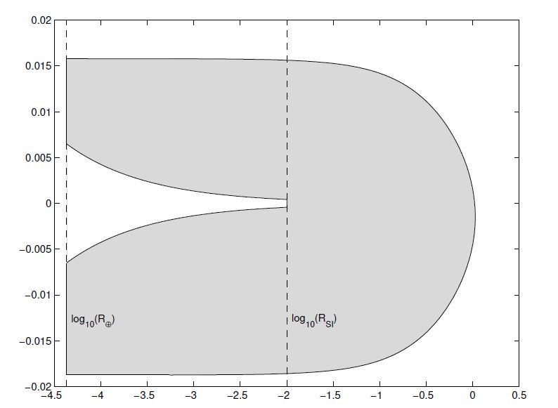
By associating the analyzed assumption and the hypothesis of a non-interstellar object, the resulting admissible region has a shape which is a consequence of the intersections between the zero level curves $\mathcal{E_{\oplus}}= 0$ and $\mathcal{E_{\odot}}= 0$. These intersections are meaningful only if $\rho \in [R_{\oplus},R_{SI}]$. It can be proved that if $\rho \in [R_{\oplus},R_{SI}]$ and $\mathcal{E_{\oplus}}\leq 0$, then also $\mathcal{E_{\odot}}\leq 0$. Therefore, the region of the solar system orbits excluding the satellites of the Earth does not have more connected components than the region satisfying only the condition $\mathcal{E_{\odot}} \leq 0$. This is a property which is valid only for the Earth, not for whatever planet.
An example of admissible region is shown in Figure 1:
The third assumption can generate the so-called “tiny object boundary”. The size of the object is related to its absolute magnitude. If the object is assumed to be large, its absolute magnitude $H(\rho)$ will be lower than some maximum value $H_{max}$. $H(\rho)$ depends on the distance by means of the relation
\[H(\rho)=h-5\log_{10}{\rho}-x(\rho),\]where $h$ is the apparent magnitude and $x(\rho)$ is a correction accounting for the distance from the Sun and the phase effect. If $\rho$ is small enough, this correction can be taken equal to a constant $x_0$ not depending on $\rho$. With this approximation, we have:
\[\log_{10}{\rho}\geq \frac{h-H_{max}-x_0}{5}=\log_{10}{\rho_H},\]and the tiny object boundary is given by $\rho=\rho_H$. If $\rho_H$ is larger than $R_{SI}$, the admissible region will be characterized by a boundary given by an outer part, corresponding to the zero level curve $\mathcal{E_{\odot}}= 0$ and by an inner part given by the tiny object boundary.
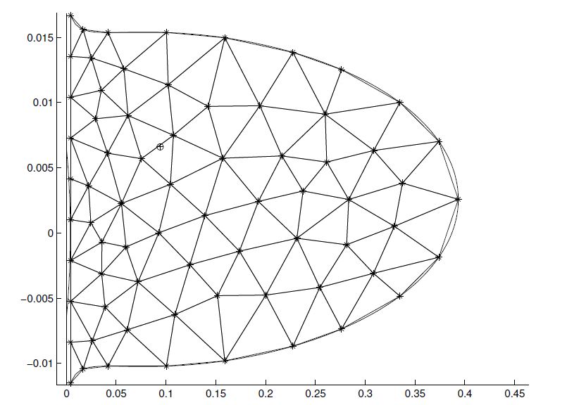
The admissible region can be sampled by means of the so-called Delaunay triangulation. This can be adopted if the considered domain $\mathcal{D}$ is convex. It consists in the definition of the pair $(\Pi,\tau)$, where $\Pi={P_1…P_N}$ is the set of nodes and $\tau={T_1…T_k}$ is the set of triangles with vertexes in $\Pi$, such that:
- $\bigcup_{i=1,k}T_i=\mathcal{D}$
- for each $i\neq j$, $T_i\bigcap T_j$ is either empty or a vertex or an edge.
To each triangulation, it is possible to associate a minimum angle, which is the minimum among the angles of all the triangles $T_i$. The Delaunay triangulation is a particular triangulation characterized by the following properties:
- it maximizes the minimum angle;
- it minimizes the maximum circumcircle;
- for each triangle $T_i$, the interior part of its circumcircle does not contain any nodes of the triangulation.
The admissible region is not generally convex. However, it is possible to sample its boundary by imposing nodes as much as possible equispaced. At this point, having these nodes as input, there will be a triangulation that maximizes the minimum angle. Thus, it will be possible to adopt a Delaunay-similar triangulation, such that only the third property could be non-respected. A sampled admissible region is shown in Figure 2:
Once the triangulation is performed, each node will correspond to an orbit that can be associated to a degenerate covariance matrix and both of them can be propagated to the epoch of a second attributable to check the compatibility of the observations.
Linkage with the Keplerian Integrals
The first integrals of Kepler’s motion can be used to write an univariate polynomial equation in the unknown quantity $\rho$ for the initial orbit determination (IOD) problem.
- Taff and Hall (1977) derive the conservation of the angular momentum and the energy to write equations for the linkage (non-polynomial formulation) ;
- Gronchi, Dimare, Milani (2010) derive a polynomial formulation from the conservarion of the angular momentum and the energy conservation (polynomial in $\rho$ of degree 48);
- Gronchi, Farnocchia, Dimare (2011) use in place of the energy the Laplace-Lenz vector projected along a suitable direction (polynomial in $\rho$ of degree 20);
- Gronchi, Baù, Marò (2015) significantly improve the previous results by considering a suitable combination of the first integrals and the conservation of the angular momentum (polynomial in $\rho$ of degree 9).
Therefore, the first step is to remember the first integrals of Kepler’s motion. The Kepler’s problem is given by
\[\ddot{\boldsymbol{r}}= -\mu\frac{\boldsymbol{r}}{|\boldsymbol{r}|^3}\]with $\boldsymbol{r}\in\mathbb{R}^3$ and $\mu>0$. This problem has these well-known integrals of motion:
- Angular Momentum: \(\boldsymbol{c} = \boldsymbol{r}\times\dot{\boldsymbol{r}},\)
- Energy: $\mathcal{E}=\cfrac{1}{2}\hspace{-1mm}\mid\hspace{-1mm}\dot{\boldsymbol{r}}\hspace{-1mm}\mid^2-\cfrac{\mu}{\mid\boldsymbol{r}\mid},$
- Laplace-Lenz vector: $\boldsymbol{L} = \cfrac{1}{\mu}\dot{\boldsymbol{r}}\times\boldsymbol{c} - \cfrac{\boldsymbol{r}}{\mid\boldsymbol{r}\mid},$
with the dependency relations
\[\boldsymbol{L}\cdot\boldsymbol{c} = 0,\] \[2|\boldsymbol{c}|^2\mathcal{E} + \mu^2\left(1-|\boldsymbol{L}|^2\right) = 0.\]In this way, given an attributable $\mathcal{A}$, the angular momentum vector can be written as a polynomial function of the radial distance $\rho$ and velocity $\dot{\rho}$
\[\boldsymbol{c}(\rho,\dot{\rho}) = \boldsymbol{D}\dot{\rho} + \boldsymbol{E}\rho^2+\boldsymbol{F}\rho + \boldsymbol{G},\]with
\[\boldsymbol{D} = \boldsymbol{q}\times \boldsymbol{e}^\rho,\quad \boldsymbol{E} = \boldsymbol{e}^\rho\times\boldsymbol{e}^\bot,\quad \boldsymbol{F}=\boldsymbol{q}\times\boldsymbol{e}^\bot + \boldsymbol{e}^\rho\times\dot{\boldsymbol{q}},\quad\boldsymbol{G}=\boldsymbol{q}\times\dot{\boldsymbol{q}},\]where
\[\boldsymbol{e}^\bot = \dot{\alpha}\cos\delta\boldsymbol{e}^\alpha+\dot{\delta}\boldsymbol{e}^\delta,\]Similarly, the expression of the energy is
\[\mathcal{E}(\rho,\dot{\rho}) = \frac{1}{2}|\dot{\boldsymbol{r}}|^2-\frac{\mu}{|\boldsymbol{r}|},\]and the Laplace-Lenz vector is given by:
\[\mu\boldsymbol{L}(\rho,\dot{\rho}) = \left(|\dot{r}|^2-\frac{\mu}{|\boldsymbol{r}|}\right)\boldsymbol{r}-(\dot{\boldsymbol{r}}\cdot\boldsymbol{r})\dot{\boldsymbol{r}},\]where
\[\mid\boldsymbol{r}\mid = \sqrt{\rho^2 + 2(\boldsymbol{q}\cdot\boldsymbol{e}^\rho)\rho + \mid\boldsymbol{q}\mid^2},\] \[\mid\dot{\boldsymbol{r}}\mid = \dot{\rho}^2 + (\dot{\alpha}^2\cos^2\delta+\dot{\delta}^2)\rho^2 + 2\dot{\boldsymbol{q}}\cdot\boldsymbol{e}^\rho + 2\dot{\boldsymbol{q}}\cdot\boldsymbol{e}^\bot\rho + \mid\dot{\boldsymbol{q}}\mid^2,\] \[\dot{\boldsymbol{r}}\cdot\boldsymbol{r} = \rho\dot{\rho} + (\dot{\boldsymbol{q}}\cdot\boldsymbol{e}^\rho+\boldsymbol{q}\cdot\boldsymbol{e}^\bot)\rho + \dot{\boldsymbol{q}}\cdot\boldsymbol{q},\]Method in Gronchi, Baù, Marò (2015)
Given the attributables $\mathcal{A}_1$, $\mathcal{A}_2$ at times $\bar{t}_1$, $\bar{t}_2$, assume they refer to the same observed body and consider the system
\[\boldsymbol{c}_1 = \boldsymbol{c}_2,\quad \boldsymbol{L}_1 = \boldsymbol{L}_2,\quad \mathcal{E}_1 = \mathcal{E}_2,\]of 7 algebraic equations in the 4 unknowns ($\rho_1,\,\rho_2,\,\dot{\rho}_1,\,\dot{\rho}_2$). The goal is to search for a polynomial system, consequence of the above conservation laws, which leads to a univariate polynomial equation with the lowest possible degree.
From the conservation of the angular momentum ($\boldsymbol{c}_1 = \boldsymbol{c}_2$) projected onto the following vectors
\[\boldsymbol{D}_1\times\boldsymbol{D}_2,\quad \boldsymbol{D}_1\times(\boldsymbol{D}_1\times\boldsymbol{D}_2),\quad \boldsymbol{D}_2\times(\boldsymbol{D}_1\times\boldsymbol{D}_2),\quad\]where $\boldsymbol{D}_j = \boldsymbol{q}_j\times\boldsymbol{e}_j^\rho$, we get, respectively
\[q(\rho_1,\rho_2) = 0,\] \[|\boldsymbol{D}_1\times\boldsymbol{D}_2|^2\dot{\rho}_1 - \boldsymbol{J}(\rho_1,\rho_2)\cdot\boldsymbol{D}_2\times(\boldsymbol{D}_1\times\boldsymbol{D}_2) = 0,\] \[|\boldsymbol{D}_1\times\boldsymbol{D}_2|^2\dot{\rho}_2 - \boldsymbol{J}(\rho_1,\rho_2)\cdot\boldsymbol{D}_1\times(\boldsymbol{D}_1\times\boldsymbol{D}_2) = 0,\]with $q$ a quadratic polynomial and $\boldsymbol{J}(\rho_1,\rho_2)=\boldsymbol{E}_2\rho_2^2-\boldsymbol{E}_1\rho_1^2+\boldsymbol{F}_2\rho_2-\boldsymbol{F}_1\rho_1+\boldsymbol{G}_2-\boldsymbol{G}_1$. The last two equations allow us to eliminate the variables $\dot{\rho}_1$ and $\dot{\rho}_2$ respectively.
The equations
\[\boldsymbol{L}_1 = \boldsymbol{L}_2,\quad\mathcal{E}_1 = \mathcal{E}_2\]are algebraic but not polynomial, due to the terms $\mu/\hspace{-1mm}\mid\hspace{-1mm}\boldsymbol{r}_j\mid$. However, we can consider the vector:
\[\boldsymbol{\xi}=\left[\mu(\boldsymbol{L}_1-\boldsymbol{L}_2) - (\mathcal{E}_1\boldsymbol{r}_1-\mathcal{E}_2\boldsymbol{r}_2)\right]\times(\boldsymbol{r}_1-\boldsymbol{r}_2)\]and note that
- in $\boldsymbol{\xi}$ the terms $\mu/\hspace{-1mm}\mid\hspace{-1mm}\boldsymbol{r}_j\mid$ are disappeared;
- in $\boldsymbol{\xi}$ the monomials with highest degree (i.e. 6) in $\rho_1$, $\rho_2$ are all multiplied by $\boldsymbol{e}_1^\rho\times\boldsymbol{e}_2^\rho$;
- if $q=0$, then $\boldsymbol{\xi}\parallel\boldsymbol{c}$, where $\boldsymbol{c} = \boldsymbol{c}_1 = \boldsymbol{c}_2$.
Therefore, we want to study the polynomial system
\[q=0,\quad \boldsymbol{\xi}=\boldsymbol{0}.\]Generically $(\boldsymbol{q}_1-\boldsymbol{q}_2)\cdot\boldsymbol{e}_1^\rho\times\boldsymbol{e}_2^\rho\neq0$ and, since $\boldsymbol{\xi}\cdot(\boldsymbol{r}_1-\boldsymbol{r}_2)=0$:
\[\boldsymbol{\xi} = \boldsymbol{0} \Longleftrightarrow \boldsymbol{\xi}\cdot\boldsymbol{e}_1^\rho = \boldsymbol{\xi}\cdot\boldsymbol{e}_2^\rho = 0.\]We introduce the polynomials (with degree 5):
\[p_1 = \boldsymbol{\xi}\cdot\boldsymbol{e}_1^\rho, \quad p_2 =\boldsymbol{\xi}\cdot\boldsymbol{e}_2^\rho\]and we are left with the bivariate system
\[q=p_1=p_2=0.\]Theorem
The equations $q=p_1=p_2=0$ can be reduced to a system of two univariate polynomials of degree 10,
such that
\[\mathfrak{u}= \text{gcd}(\mathfrak{u}_1, \mathfrak{u}_2)\]has degree 9.
The polynomials $\mathfrak{u}_1$ and $\mathfrak{u}_2$ are defined by
\[\mathfrak{u}_1=\text{Res}(p_1,q,\rho_1),\quad \mathfrak{u}_2=\text{Res}(p_2,q,\rho_1)\]where $\text{Res}()$ denotes the resultant.
If we consider the auxiliary variable $u$ defined by the relation
\[u|\boldsymbol{r}|=\mu\]then the Keplerian integrals can be viewed as polynomials in the variables $\rho$, $\dot{\rho}$ and $u$ by writing $u$ in place of $\mu/\hspace{-1mm}\mid\hspace{-1mm}\boldsymbol{r}\mid$. In particular, we obtain
\[\mu\boldsymbol{L} = \left(\mid\dot{\boldsymbol{r}}\hspace{-1mm}\mid\hspace{-1mm}^2-u\right)\boldsymbol{r}-\left(\dot{\boldsymbol{r}}\cdot\boldsymbol{r}\right)\dot{\boldsymbol{r}},\quad\mathcal{E}=\frac{1}{2}\hspace{-1mm}\mid\hspace{-1mm}\dot{\boldsymbol{r}}\hspace{-1mm}\mid\hspace{-1mm}^2-u.\]However, the polynomial system of 9 equations
\[\boldsymbol{c}_1 = \boldsymbol{c}_2,\quad \mu\boldsymbol{L}_1 = \mu\boldsymbol{L}_2,\quad \mathcal{E}_1 = \mathcal{E}_2,\quad u_1^2|\boldsymbol{r}_1|^2=\mu^2,\quad u_2^2|\boldsymbol{r}_2|^2=\mu^2\]with unknowns $\rho_1$, $\rho_2$, $\dot{\rho}_1$, $\dot{\rho}_2$, $u_1$ and $u_2$ is generically not consistent.
Gronchi, Baù and Milani (2017) proved that if we drop the last two equations, then we obtain a consistent polynomial system
\[\boldsymbol{c}_1 = \boldsymbol{c}_2,\quad \mu\boldsymbol{L}_1 = \mu\boldsymbol{L}_2,\quad \mathcal{E}_1 = \mathcal{E}_2,\]in the variables $\rho_1$, $\rho_2$, $u_1$, $u_2$, $\dot \rho_1$ and $\dot\rho_2$. Moreover, the univariate polynomial
\[\mathfrak{u}= \text{gcd}(\mathfrak{u}_1, \mathfrak{u}_2)\]of degree 9 has the minimum degree among the polynomials in $\rho_1$ or $\rho_2$ contained in the ideal:
\[I = \langle\boldsymbol{c}_1 - \boldsymbol{c}_2,\, \mu(\boldsymbol{L}_1 - \boldsymbol{L}_2),\, \mathcal{E}_1 - \mathcal{E}_2\rangle\subseteq \mathbb{R}\left[\rho_1,\rho_2,\dot{\rho}_1,\dot{\rho}_2,u_1,u_2\right].\]More precisely, the following result holds true:
Theorem
For generic data $\mathcal{A}_1,\mathcal{A}_2,\boldsymbol{q}_1,\boldsymbol{q}_2,\dot{\boldsymbol{q}}_1,\dot{\boldsymbol{q}}_2$ we can find (by hand) a set of polynomials
that is a Gröbner basis of the ideal $I$ for the lexicographic order
\[\dot{\rho}_1\succ\dot{\rho}_2\succ u_1\succ u_2\succ\rho_1\succ\rho_2,\]and such that
\[\mathfrak{g}_6=\mathfrak{u}\]Selection of the solutions
We consider an example with the system
\[\boldsymbol{c}_1 = \boldsymbol{c}_2,\quad \mathcal{E}_1 = \mathcal{E}_2.\]The attributables $\mathcal{A}_1$, $\mathcal{A}_2$ give 8 scalar data, thus the problem is overdetermined: from a non-spurious solution $\rho_1$, $\rho_2$ we obtain the same values of the elements $a$, $e$, $I$, $\Omega$ at times
\[\tilde{t}_j = \bar{t}_j+\frac{\rho_j}{c},\quad j=1,2,\]corrected by aberration, but we must check that the compatibility conditions
\[\omega_1 = \omega_2,\quad\ell_1=\ell_2+n(\tilde{t}_1-\tilde{t}_2),\]are verified within some threshold, where $n$ is the mean motion of the observed body.
Covariance of the solutions
Given \(A=(\mathcal{A}_1\), \(\mathcal{A}_2)\) with covariance matrices \(\Gamma_{\mathcal{A}_1}\), \(\Gamma_{\mathcal{A}_2}\), let
\[\boldsymbol{R}=\boldsymbol{R}(\boldsymbol{A}) = \left(\mathcal{R}_1(\boldsymbol{A}),\mathcal{R}_2(\boldsymbol{A})\right),\quad\mathcal{R}_j=(\rho_j,\dot{\rho}_j)\quad j=1,2\]be a solution of
\[\boldsymbol{\Phi}(\boldsymbol{R};\boldsymbol{A})=\boldsymbol{0},\quad \boldsymbol{\Phi}(\boldsymbol{R};\boldsymbol{A})= \left(\begin{matrix} \boldsymbol{D}_1\dot{\rho}_1 - \boldsymbol{D}_2\dot{\rho}_2 - \boldsymbol{J}(\rho_1,\rho_2)\\ \mathcal{E}_1(\rho_1,\dot{\rho}_1)-\mathcal{E}_2(\rho_2,\dot{\rho}_2) \end{matrix} \right).\]If both $(\mathcal{A}_1,\mathcal{R}_1(\boldsymbol{A}))$, $(\mathcal{A}_2,\mathcal{R}_2(\boldsymbol{A}))$ give bounded orbits at times $\tilde{t}_1$, $\tilde{t}_2$, then we can compute the corresponding Keplerian elements. We introduce the map
\[(\mathcal{A}_1,\mathcal{A}_2) = \boldsymbol{A} \longmapsto \Psi(A) = (\mathcal{A}_1,\mathcal{R}_1,\Delta_{1,2}),\]giving the orbit $(\mathcal{A}_1,\mathcal{R}_1(\boldsymbol{A}))$ in spherical coordinates at time $\tilde{t}_1$, together with the difference
\[\Delta_{1,2}(\boldsymbol{A}) = (\Delta\omega,\Delta\ell) = (\omega_2 - \omega_1,\, \ell_2 + n(\tilde{t}_1 -\tilde{t}_2) - \ell_1) ,\]in the angular elements which are not constrained by the angular momentum and the energy integrals. By the covariance propagation rule we have
\[\Gamma_{\boldsymbol{\Psi}(\boldsymbol{A})}=\frac{\partial \boldsymbol{\Psi}}{\partial \boldsymbol{A}}\Gamma_{\boldsymbol{A}}\left[\frac{\partial \boldsymbol{\Psi}}{\partial \boldsymbol{A}}\right]^T\]where
\[\frac{\partial \boldsymbol{\Psi}}{\partial \boldsymbol{A}} = \left( \begin{matrix} I & 0\\ \frac{\partial \mathcal{R}_1}{\partial \mathcal{A}_1} & \frac{\partial \mathcal{R}_1}{\partial \mathcal{A}_2}\\ \frac{\partial \Delta_{1,2}}{\partial \mathcal{A}_1} & \frac{\partial \Delta_{1,2}}{\partial \mathcal{A}_2}\\ \end{matrix} \right) \quad\text{and}\quad \Gamma_{\boldsymbol{A}} = \left( \begin{matrix} \Gamma_{\mathcal{A}_1} & 0\\ 0 & \Gamma_{\mathcal{A}_2}\\ \end{matrix} \right).\]Identification of attributables
The problem is to decide whether the two sets of observations defining $\mathcal{A}_1$, $\mathcal{A}_2$ can belong to the same Solar system body. Forthis purpose, we need to check whether the failure of condition
\[\Delta_{1,2}(\boldsymbol{A}) = \boldsymbol{0}\]is acceptable, that is if $\Delta\omega$ and $\Delta l$ are compatible with the observational errors. Take the marginal covariance matrix:
\[\Gamma_{\Delta_{1,2}}= \frac{\partial \Delta_{1,2}}{\partial \boldsymbol{A}}\Gamma_{\boldsymbol{A}}\left[\frac{\partial \Delta_{1,2}}{\partial \boldsymbol{A}}\right]^T,\]the inverse matrix $C^{\Delta_{1,2}} = \Gamma_{\Delta_{1,2}}^{-1}$ defines a norm $||\cdot||_*$ in the $(\Delta\omega,\Delta\ell)$ plane, allowing to test the identification of $\mathcal{A}_1$ and $\mathcal{A}_2$.
This linkage method also allows to assign an uncertainty to the preliminary orbits that we compute.
Joining three TSAs
Given 3 TSAs at 3 mean epochs, the conservation of the angular momentum is enough to obtain a finite number of orbits.
Consider the polynomial equations:
\[\boldsymbol{c}_1 = \boldsymbol{c}_2,\quad \boldsymbol{c}_2 = \boldsymbol{c}_3,\quad \boldsymbol{c}_3 = \boldsymbol{c}_1,\]in the unknowns $\rho_1,\dot{\rho}_1,\rho_2,\dot{\rho}_2,\rho_3,\dot{\rho}_3$. The previous equations are redundant: if $\boldsymbol{D}_1\times\boldsymbol{D}_2\cdot\boldsymbol{D}_3\neq0$ they are equivalent to
\[\begin{aligned} &(\boldsymbol{c}_1-\boldsymbol{c}_2)\cdot\boldsymbol{D}_1\times\boldsymbol{D}_2 = 0,\\[1.5ex] &(\boldsymbol{c}_2-\boldsymbol{c}_3)\cdot\boldsymbol{D}_2\times\boldsymbol{D}_3 = 0,\\[1.5ex] &(\boldsymbol{c}_3-\boldsymbol{c}_1)\cdot\boldsymbol{D}_3\times\boldsymbol{D}_1 = 0,\\[1.5ex] &(\boldsymbol{c}_1-\boldsymbol{c}_2)\cdot\boldsymbol{D}_1\times(\boldsymbol{D}_1\times\boldsymbol{D}_2) = 0,\\[1.5ex] &(\boldsymbol{c}_2-\boldsymbol{c}_3)\cdot\boldsymbol{D}_2\times(\boldsymbol{D}_2\times\boldsymbol{D}_3) = 0,\\[1.5ex] &(\boldsymbol{c}_3-\boldsymbol{c}_1)\cdot\boldsymbol{D}_3\times(\boldsymbol{D}_3\times\boldsymbol{D}_1) = 0. \end{aligned}\]The first three equations depends only on the radial distance. In fact, they correspond to the system
\[\boldsymbol{J}_{12}\cdot\boldsymbol{D}_1\times\boldsymbol{D}_2 = 0,\quad \boldsymbol{J}_{23}\cdot\boldsymbol{D}_2\times\boldsymbol{D}_3 = 0,\quad \boldsymbol{J}_{23}\cdot\boldsymbol{D}_2\times\boldsymbol{D}_3 = 0\]which can be written as
\[\begin{aligned} q_3 &= a_3\rho_2^2 + b_3\rho_1^2 + c_3\rho_2 + d_3\rho_1 + e_3 = 0,\\[1.5ex] q_1 &= a_1\rho_3^2 + b_1\rho_2^2 + c_1\rho_3 + d_1\rho_2 + e_1 = 0,\\[1.5ex] q_2 &= a_2\rho_1^2 + b_2\rho_3^2 + c_2\rho_1 + d_2\rho_3 + e_2 = 0, \end{aligned}\]where
\[\begin{gather} a_3 = \boldsymbol{E}_2\cdot\boldsymbol{D}_1\times\boldsymbol{D}_2, \quad b_3 = -\boldsymbol{E}_1\cdot\boldsymbol{D}_1\times\boldsymbol{D}_2,\\[1.5ex] c_3 = \boldsymbol{F}_2\cdot\boldsymbol{D}_1\times\boldsymbol{D}_2, \quad d_3 = -\boldsymbol{F}_1\cdot\boldsymbol{D}_1\times\boldsymbol{D}_2, \\[1.5ex] c_3 = (\boldsymbol{G}_2 -\boldsymbol{G}_1)\cdot\boldsymbol{D}_1\times\boldsymbol{D}_2, \end{gather}\]and the other coefficients $a_j$, $b_j$, $c_j$, $d_j$, $e_j$ for $j=1,2$, have similar expressions, obtained by cycling the indexes.
To eliminate $\rho_1, \rho_3$ we first compute the resultant
\[r = \text{Res}(q_3,q_2,\rho_1),\]which depends only on $\rho_2,\rho_3$. Then we compute the resultant
\[\mathfrak{q} = \text{Res}(r,q_1,\rho_3),\]which is a univariate polynomial of degree 8 in the variable $\rho_2$.
Therefore, to get the solution of the conservation of the angular momentum, we
- search for the roots $\bar{\rho}_2$ of $\mathfrak{q}(\rho_2)$,
- compute the corresponding values of $\bar{\rho}_3$ from system $r(\rho_3,\bar{\rho}_2) = q_1(\rho_3,\bar{\rho}_2) = 0$,
- compute the corresponding values of $\bar{\rho}_1$ from system $q_3(\rho_1,\bar{\rho}_2) = q_2(\bar{\rho}_3,\rho_1) = 0$.
- compute the radial velocities $\dot \rho_j$:
A particular solution can be obtained by searching for values $\rho_j$, $\dot{\rho}_j$ such that
\[\boldsymbol{c}_j(\rho_j,\dot{\rho}_j)=\boldsymbol{0},\quad j=1,2,3.\]Finally, we can discard solutions by using compatibility conditions, as for the case with two TSAs.