Generalization of a method by Mossotti for initial orbit determination
In 1816 Ottaviano F. Mossotti introduced a method for initial orbit determination of a solar system body employing four observations (the observations of asteroids of that epoch were no more than one per night, therefore the time interval between two of them covered a few days), assumed geocentric, that allows to write linear equations for the computation of the orbital angular momentum [Mossotti 1816]. Then the orbit can be reconstructed, e.g. by Gibbs’ method. This procedure has the advantage to avoid the computation of the roots of the eight degree polynomial appearing in the classical methods, which use only three observations but can give rise to multiple solutions.
This method has been reviewed in [Celletti et al. 2006], where the authors state that the computation of the solution can be seriously affected by the observational errors. It is important to note that in the early XIX century Linear Algebra had not been developed so Mossotti’s original method can be deduced and rewritten in a more compact and easily way.
The original method
Mossotti’s method leads to a set of linear equations for the components of $\boldsymbol{c}_{\oplus} - \boldsymbol{c}$ where
- $\boldsymbol{c}_{\oplus}$ is the angular momenta of the Earth,
- $\boldsymbol{c}$ is the angular momentum of the body of the solar system whose orbit we want to determine.
The observations are supposed to be made from the center of the Earth and we shall assume that the observed body is an asteroid.
Units and preliminary definitions
We use the rescaled time $\theta$, defined by
\[\theta = t\sqrt{G(m_\odot+m_\oplus)} = t\sqrt{Gm_\odot\left(1+\frac{m_\oplus}{m_\odot}\right)},\]where
- $m_\oplus$ is the masses of the Earth,
- $m_\odot$ the masses of the Sun,
- $G$ is Newton’s gravitational constant.
We also use $\kappa = \sqrt{Gm_\odot}$ to denote Gauss’ constant.
In the following we assume that
\[\theta \approx \kappa t,\]neglecting the constant ${m_\oplus}/{m_\odot}$.
We take three of the four observations, at epochs $t_1<t_2<t_3$, and set
\[\theta_{ij} = \kappa (t_j - t_i),\]and we introduce the vector
\[\boldsymbol{\theta} = \left( \begin{matrix} \theta_{23}\\ \theta_{31}\\ \theta_{12} \end{matrix} \right).\]For the orbital angular momenta of the asteroid and the Earth we introduce their unit vectors
\[\hat{\boldsymbol{c}} = \frac{\boldsymbol{c}}{c}, \qquad \hat{\boldsymbol{c}}_\oplus = \frac{\boldsymbol{c}_\oplus}{c_\oplus},\]where $c=|\boldsymbol{c}|$, $c_\oplus=|\boldsymbol{c}_\oplus|$, being $|\boldsymbol{x}|$ the Euclidean norm of a vector $\boldsymbol{x}$.
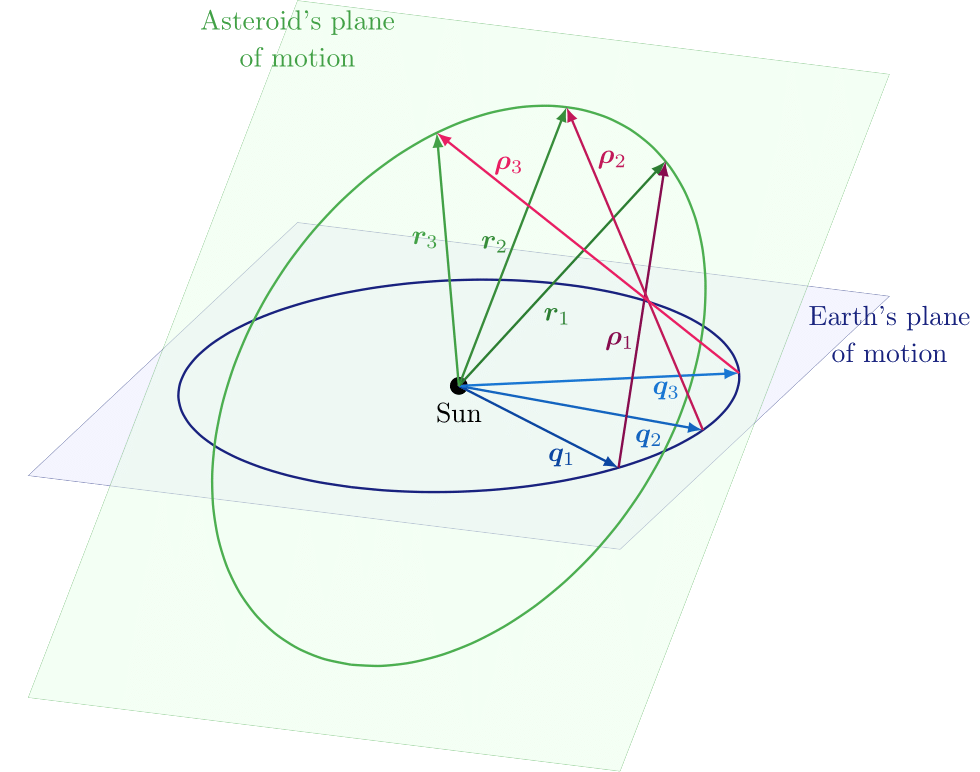
We also write $\boldsymbol{r}_i$ and $\boldsymbol{q}_i$ for the heliocentric positions of the asteroid and the Earth at the three epochs $t_i$ ($i=1,2,3$), use $\boldsymbol{\rho}_i = \boldsymbol{r}_i - \boldsymbol{q}_i$ for the geocentric position of the asteroid, and introduce the unit vectors
\[\hat{\boldsymbol{q}}_i = \frac{\boldsymbol{q}_i}{q_i},\qquad \hat{\boldsymbol{\rho}}_i = \frac{\boldsymbol{\rho}_i}{\rho_i},\qquad i=1,2,3,\]where $q_i=|\boldsymbol{q}_i|$, $\rho_i=|\boldsymbol{\rho}_i|$. Finally, we denote the parameters of the orbits of the asteroid and the Earth by
\[p = a(1-e^2), \qquad p_\oplus = a_\oplus(1-e_\oplus^2),\]where $a$, $a_\oplus$, and $e$, $e_\oplus$ stands for the semimajor axes and eccentricities. Note that
\[p\kappa^2 = c^2,\qquad p_\oplus\kappa^2 = c_\oplus^2.\]For our purpose, let us introduce the matrices
\[\begin{aligned} P &= (\boldsymbol{\rho}_1\, | \, \boldsymbol{\rho}_2 \, | \, \boldsymbol{\rho}_3),\\ Q &= (\boldsymbol{q}_1\, | \, \boldsymbol{q}_2 \, | \, \boldsymbol{q}_3),\\ R &= P + Q = (\boldsymbol{r}_1\, | \, \boldsymbol{r}_2 \, | \, \boldsymbol{r}_3), \end{aligned}\]where $(\boldsymbol{x}_1 \,|\, \boldsymbol{x}_2 \,|\, \boldsymbol{x}_3)$ is the matrix whose columns are the vectors $\boldsymbol{x}_j$. The corresponding adjugate matrices are
\[\begin{aligned} \text{adj}(P) &= \left(\boldsymbol{\rho}_2\times\boldsymbol{\rho}_3\,|\, \boldsymbol{\rho}_3\times\boldsymbol{\rho}_1\,|\, \boldsymbol{\rho}_1\times\boldsymbol{\rho}_2\right)^{\,t},\\ % \text{adj}(Q) &= \left(\boldsymbol{q}_2\times\boldsymbol{q}_3\,|\, \boldsymbol{q}_3\times\boldsymbol{q}_1\,|\, \boldsymbol{q}_1\times\boldsymbol{q}_2\right)^{\,t},\\ % \text{adj}(R) &= \left(\boldsymbol{r}_2\times\boldsymbol{r}_3\,|\, \boldsymbol{r}_3\times\boldsymbol{r}_1\,|\, \boldsymbol{r}_1\times\boldsymbol{r}_2\right)^t.\\ \end{aligned}\]where the superscript $t$ stands for transposition.
Geometric relations
We recall the following property, which holds for any square matrix $M$:
\[M\,\text{adj}(M) = \text{adj}(M)\,M = \text{det}(M)\,I,\]where $I$ is the identity matrix.
The rank of the matrices $Q$ and $R$ is $2$, since each triple ${\boldsymbol{q}_1, \boldsymbol{q}_2,\boldsymbol{q}_3}$ and ${\boldsymbol{r}_1, \boldsymbol{r}_2, \boldsymbol{r}_3}$ is made by coplanar vectors and we assume that
\[\boldsymbol{q}_i\times\boldsymbol{q}_j\neq \boldsymbol{0}, \qquad \boldsymbol{r}_i\times\boldsymbol{r}_j\neq \boldsymbol{0}, \qquad i\neq j,\]see Figure 1. This implies
\[Q\,\text{adj}(Q)= 0, \qquad R\,\text{adj}(R) = 0.\]Then, we introduce the vectors
\[\boldsymbol{T} = \begin{pmatrix} T_1\\ T_2\\ T_3 \end{pmatrix} = \frac{1}{\sqrt{p_\oplus}} \text{adj}(Q)\hat{\boldsymbol{c}}_\oplus, \boldsymbol{\tau} = \begin{pmatrix} \tau_1\\ \tau_2\\ \tau_3 \end{pmatrix} = \frac{1}{\sqrt{p}} \text{adj}(R)\hat{\boldsymbol{c}},\qquad\]so
\[Q\,\boldsymbol{T}= 0, \qquad R\,\boldsymbol{\tau} = 0.\]and recalling that $ R = P+Q$ we have
\[P\boldsymbol{\tau} = Q(\boldsymbol{T}-\boldsymbol{\tau}).\]We will refer to this last equation as (1).
Since the angular momenta $\boldsymbol{c}$, $\boldsymbol{c}_\oplus$ are respectively orthogonal to the orbital planes of the asteroid and the Earth, we have
\[\boldsymbol{c}\cdot\boldsymbol{r}_i = \boldsymbol{c}\cdot(\boldsymbol{q}_i+\boldsymbol{\rho}_i)= 0,\quad \boldsymbol{c}_\oplus\cdot\boldsymbol{q}_i = 0,\]which lead us to
\[\boldsymbol{c}\cdot\boldsymbol{\rho}_i = (\boldsymbol{c}_\oplus-\boldsymbol{c})\cdot\boldsymbol{q}_i,\]for $i=1,2,3$.
A linear equation
With some manipulations (see [Gronchi et al. 2021] for details) we obtain:
\[(\boldsymbol{c}_\oplus - \boldsymbol{c}) \cdot (\hat{\boldsymbol{\rho}}_i + \alpha_{ik}\hat{\boldsymbol{q}}_i ) = \varepsilon_{ijk}\frac{a_{ik}c_\oplus\rho_j}{q_j}\]we will refer to this last equation as (2), where
- $\varepsilon_{ijk}$ denotes the Levi-Civita symbol,
- $a_{ik}$ is a division of two triple products,
are known quantities and we want to determine or eliminate
- $\rho_j$,
- $\alpha_{ik} = \left(1-\cfrac{\tau_k}{T_k}\right)\cfrac{q_i}{\rho_i}$.
We can obtain an approximation of $\alpha_{ik}$ using the 2-body dynamics and eliminate $\rho_j$ using 2 different choices of the indices $i,j,k$ and combining the two equations.
Choosing $(i,j,k)=(1,2,3), (3,2,1)$ we can eliminate $\rho_2$:
\[(\boldsymbol{\gamma}-\boldsymbol{\varphi})\cdot\left(\boldsymbol{c}_\oplus-\boldsymbol{c}\right) = 0,\]see [Gronchi et al. 2021] for details.
Mossotti’s equation
With the aim of writing two independent linear equations, all the four observations are used. If we consider two different choices of the three observations, out of the available four, we obtain the system
\[\begin{aligned} &(\boldsymbol{\gamma}_1-\boldsymbol{\varphi}_1)\cdot\left(\boldsymbol{c}_\oplus-\boldsymbol{c}\right) = 0,\\[1.5ex] &(\boldsymbol{\gamma}_2-\boldsymbol{\varphi}_2)\cdot\left(\boldsymbol{c}_\oplus-\boldsymbol{c}\right) = 0, \end{aligned}\]where the subscripts $1$, $2$ of $boldsymbol{\gamma}$ and $\boldsymbol{\varphi}$ refer to the two triplets of observations. Set
\[\boldsymbol{w} = (\boldsymbol{\gamma}_1-\boldsymbol{\varphi}_1)\times(\boldsymbol{\gamma}_2-\boldsymbol{\varphi}_2)\]and assume $\boldsymbol{w}\neq\boldsymbol{0}$. Then the general solution of the previuos system has the form
\[\boldsymbol{c}_\oplus - \boldsymbol{c} = \lambda\boldsymbol{w},\]with $\lambda\in\mathbb{R}$, giving the direction of $\boldsymbol{c}_\oplus - \boldsymbol{c}$.
In order to determine $\lambda$ we use an extra linear equation constructed easily from the previous computations.
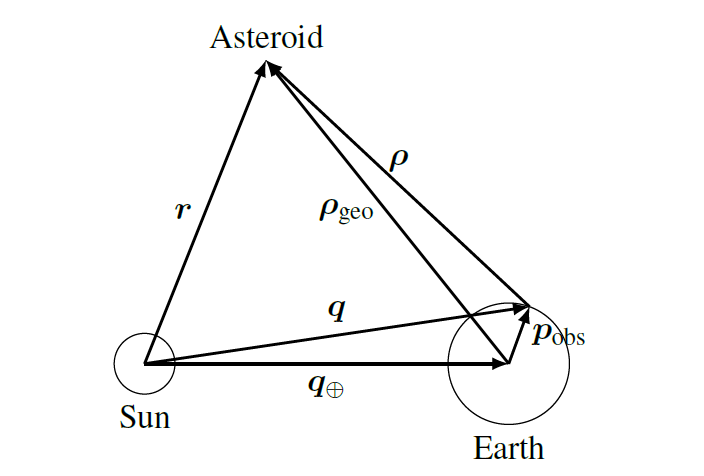
The topocentric version of the method
he original Mossotti method original can be generalized to topocentric observations which leads to a quadratic equation for the angular momentum $\boldsymbol{c}$. This allows us to assume that the observations are not made from the center of the Earth but from the surface allowing a much more realistic approach to the problem.
This approach is computationally more expensive than the original one but it allows to obtain better results and continues to be very fast, reducing the computational cost (see [Gronchi et al. 2021]) by more than 6 times compared to the Gauss method.
The idea of the method can be described in the same three steps of the original one, but with some differences: the linear equation that we obtain from each triplet is not homogeneous in general, therefore we obtain the following system for the difference of the angular momentum:
\[\begin{aligned} &(\boldsymbol{\gamma}_1-\boldsymbol{\varphi}_1)\cdot\left(\boldsymbol{c}_\oplus-\boldsymbol{c}\right) = D_1,\\[1.5ex] &(\boldsymbol{\gamma}_2-\boldsymbol{\varphi}_2)\cdot\left(\boldsymbol{c}_\oplus-\boldsymbol{c}\right) = D_2, \end{aligned}\]where $\boldsymbol{\gamma}_i$, $\boldsymbol{\varphi}_i$, $D_i$, $i = 1,2$ are known quantities. The general solution now is given by
\(\boldsymbol{c}_\oplus-\boldsymbol{c} = \lambda\boldsymbol{w} + \boldsymbol{g},\) with $\boldsymbol{w}$, $\boldsymbol{g}$ known vectors and $\lambda\in\mathbb{R}$. This makes quadratic the extra equation needed to find the value of $\lambda$, instead of linear.
From asteroids to space debris
The topocentric version admits a reformulation allowing to deal with space debris observations. Here the role of the geocentric position of the observer $\boldsymbol{p}_{obs}$ in the asteroid case is played by the component of the geocentric position of the observer parallel to the rotation axis of the Earth.
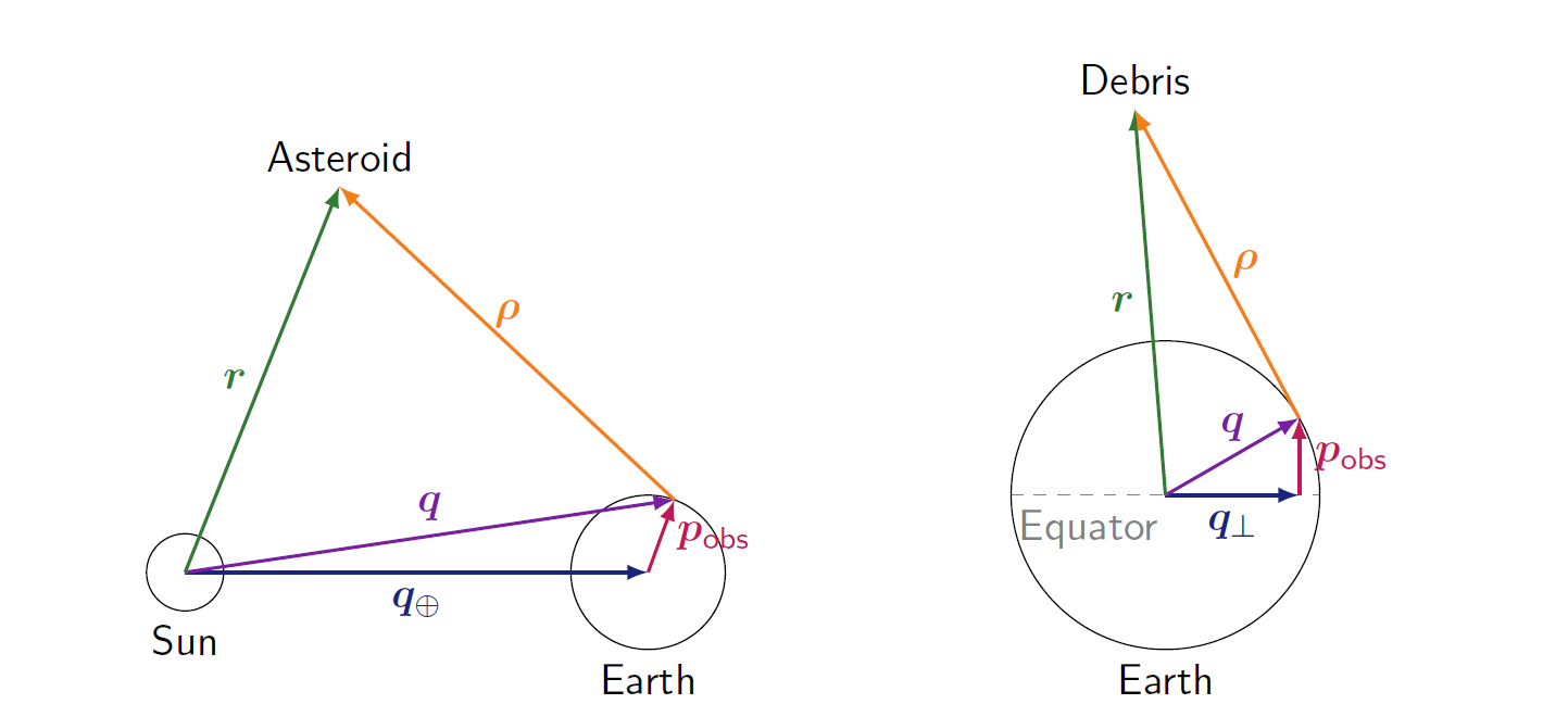
In this case the size of $\boldsymbol{p}_{obs}$ can be of the same order of the topocentric distance of the debris.