Equations of Motion for Free-Floating Robots
In this page, a derivation for the equations of motion for robotic manipulators with free-floating base is given. This derivation is mainly adapted from the following works: T.-C. Nguyen-Huynh, 2013 and Wilde et. al. 2018. Various other researchers have derived the same equations of motion (albeit sometimes with different generalized coordinates). Different researchers tend to usually use different conventions for naming the variables and frames. An effort is made here to use the most commonly used variable names. Furthermore, at certain points, the alternative terminology used by other researchers is also given so as to provide a clearer picture while reading the literature on this topic.
Usually ground-based robotic manipulator’s equations of motion contain 2 distinct sets of equations: Kinematic equations and Dynamics equations. However, for a free-floating base, the kinematics and dynamics of the manipulator are inherently coupled. This is due to the free-floating nature of the system i.e the motion of the manipulator causes a reaction on the base causing it to move which in-turn causes the manipulator to also move. Due to this, the kinematics of the manipulator contain dynamic terms which will be seen in the following sections.
The following figure shows the system under study and the conventional notations of various quantities:
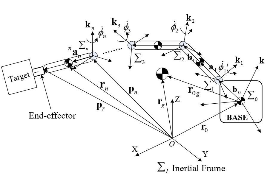
Here, the terms are as follows:
$CoM$ - Center of Mass.
$a_i$ - Position Vector from Joint to $CoM$ of Link $i$.
${}^na_n$ - Position of $CoM$ of last link w.r.t $\Sigma_n$ frame.
$b_i$ - Position Vector from $CoM$ of Link $i$ to Joint $i+1$.
$\Sigma_I$ - Inertial Frame of Reference.
$\Sigma_i$ - Link $i$ Frame of Reference.
$\Sigma_n$ - Last Link Frame of Reference.
$r_g$ - Position of $CoM$ of the System.
$r_i$ - Position of $CoM$ of link $i$.
$p_r$ - Position of End Effector from origin of Inertial frame.
$k_i$ - Unit vector along the rotation direction of Joint $i$.
$\dot{\phi}_i$ - Angular velocity of joint $i$.
$m_i$ - Mass of link $i$.
$M$ - Total mass of the system.
$L$ - Total Angular Momentum of the system.
$L_g$ - Angular Momentum About System CoM.
$P$ - Total Linear Momentum of the System.
End Effector Velocity
As the starting point for the equations of motion, the position of the end effector can be given as:
\[p_r = r_0 + b_0 + \sum_{i=1}^{n} l_i \ \ \ \ \ \ \ \ \ \ \ \ \ \ \ [1]\]where $l_i = a_i+b_i$. Differentiating equation 1 on both sides, we get the linear velocity of the end-effecter as:
\[V_r = V_0 + \omega_0 \times b_o + \sum_{i=1}^{n} \omega_i \times l_i \ \ \ \ \ \ \ \ \ \ \ \ \ \ \ [2]\]Similarly, the angular velocity of link $i$ can be given as:
\[\omega_i = \omega_0 + \sum_{j=1}^{i} k_j \dot{\phi}_i \ \ \ \ \ \ \ \ \ \ \ \ \ \ \ [3]\]Substituting equations [3] and [1] in [2], we get:
\[V_r = V_0 + \omega_0 \times (p_r - p_0) + \sum_{i=1}^{n} (k_i \times (p_r - p_i)) \dot{\phi}_i \ \ \ \ \ \ \ \ \ \ \ \ \ \ \ [4]\]The above equation ([4]) shows the relation between the end effector velocity and the base velocity and joint rates. This can be combined with the angular velocity of the last link from equation [3] and be written in the matrix as:
\[\begin{bmatrix} V_r \\ \omega_n \end{bmatrix} = J_s \begin{bmatrix} V_0 \\ \omega_0 \end{bmatrix} + J_m \dot{\phi} \ \ \ \ \ \ \ \ \ \ \ \ \ \ \ [5]\]In the above equation ([5]), the following terms are introduced:
\[\dot{\phi} = \begin{bmatrix} \dot{\phi}_1 & \dot{\phi}_2 & \dot{\phi}_3 & .... & \dot{\phi}_n \end{bmatrix}^T \in R^n\] \[J_s = \begin{bmatrix} E & -\tilde{p}_{0r} \\ 0 & E\end{bmatrix} \in R^{6 \times 6}, \ \ p_{0r} = p_r - p_0\] \[J_m = \begin{bmatrix} k_1 \times (p_r-p_1) & k_2 \times (p_r-p_2) & k_3 \times (p_r-p_3) & ... & k_n \times (p_r-p_n) \\ k_1 & k_2 & k_3 & ... & k_n \end{bmatrix} \in R^{6 \times n}\]Here, $E$ is the identity matrix and $\tilde{(.)}$ refers to the skew-symmetric form of a vector. An example of such a transformation is given below:
\[\tilde{\begin{bmatrix} x \\ y \\ z \end{bmatrix}} = \begin{bmatrix} 0 & -z & y \\ z & 0 & -x \\ -y & x & 0 \end{bmatrix}\]From equation [5] it can be seen that the end-effector state is determined using two terms. The term $J_s$ is called the jacobian matrix of the base spacecraft (sometimes also referred to as $J_b$ for the base jacobian). The therm $J_m$ is the jacobian matrix of the fixed base manipulator.
Momentum Equations
We can use $P$ and $L$ to represent the total linear and angular momentum of the spacecraft and robot manipulator system respectively. These terms can be given as:
\[P = \sum_{i=0}^{n} m_i \dot{r}_i \ \ \ \ \ \ \ \ \ \ \ \ \ \ \ [6]\] \[L = \sum_{i=0}^{n}(I_i \omega_i + r_i \times m_i \dot{r}_i) \ \ \ \ \ \ \ \ \ \ \ \ \ \ \ [7]\]Here, $I_i$ is the inertia tensor of the link $i$, $m_i$ is the mass of link $i$. All vectors are taken with respect to the inertial frame.
Using equation [4], $\dot{r}_i$ can be written as:
\[\dot{r}_i = V_0 + \omega_0 \times (r_i - p_0) + \sum_{j=1}^{i} (k_i \times (r_i - p_j)) \dot{\phi}_j \ \ \ \ \ \ \ \ \ \ \ \ \ \ \ [8]\]Substituting equations [8] and [3] in equations [6] and [7], we can obtain:
\[P = M V_0 + M \tilde{r}_{0g}^T \omega_0 + \sum_{i=1}^{n} \sum_{j=1}^{i} m_i (k_j \times (r_i-p_j)) \dot{\phi}_j \ \ \ \ \ \ \ \ \ \ \ \ \ \ \ [9]\] \[L = M \tilde{r}_{g} V_0 + (\sum_{i=0}^{n} (I_i - m_i \tilde{r}_i \tilde{r}_{0i}))\omega_0 + \sum_{i=1}^{n} \sum_{j=1}^{i} (m_i \tilde{r}_i (k_j \times (r_i-p_j)) + I_ik_j)\dot{\phi}_j \ \ \ \ \ \ \ \ \ \ \ \ \ \ \ [10]\]Here, the new terms introduced are as follows:
\(M = \sum_{i=0}^{n}m_i\)
\(r_g = \frac{\sum_{i=0}^{n}m_ir_i}{M}\) $r_g$ is the position vector of the center of mass of the system. Thereby, the following terms are defined as: $r_{0i} = r_i - r_0$, and thus, $r_{0g} = r_g - r_0$.
The momentum equations [9] and [10] can be expressed in matrix form as given by Yoshida et. al, 1993. This is shown in equation [11] below:
\[\begin{bmatrix} P \\ L \end{bmatrix} = \begin{bmatrix} ME & M \tilde{r}_{0g}^T \\ M \tilde{r}_{g} & I_w \end{bmatrix} \begin{bmatrix} V_0 \\ \omega_0 \end{bmatrix} + \begin{bmatrix} J_{Tw} \\ I_{\phi} \end{bmatrix} \dot{\phi} \ \ \ \ \ \ \ \ \ \ \ \ \ \ \ [11]\]Here, the terms $I_w$, $I_{\phi}$, and $J_{Tw}$ can be expressed as follows by utilizing the extra terms $J_{Ti}$ and $J_{Ri}$. These are given below:
\[I_w = \sum_{i=0}^{n} (I_i - m_i \tilde{r}_i \tilde{r}_{0i}) = \sum_{i=1}^{n} (I_i - m_i \tilde{r}_i \tilde{r}_{0i}) + I_0 \in R^{3 \times 3}\] \[J_{Ti} = \begin{bmatrix} \tilde{k}_1 (r_i - p_1) & \tilde{k}_2 (r_i - p_2) & \tilde{k}_3 (r_i - p_3) & ... & \tilde{k}_i (r_i - p_i) & 0 & 0 & ... & 0 \end{bmatrix}\] \[J_{Tw} = \sum_{i=1}^{n} \sum_{j=1}^{i} m_i (\tilde{k}_j (r_i - p_j)) = \sum_{i=1}^{n} m_i J_{Ti}\] \[J_{Ri} = \begin{bmatrix} k_1 & k_2 & k_3 & ... & k_i & 0 & 0 & ... & 0 \end{bmatrix}\] \[I_{\phi} = \sum_{i=1}^{n} (m_i \tilde{r}_i J_{Ti} + I_i J_{Ri}) \in R^{3 \times n}\]From here, we can continue with 2 different ways to derive expressions for linear and angular momentum (similar to equation [11]): one with the angular momentum taken around the system center of mass (CoM) and one with the angular momentum taken about the base CoM. The different conventions for computing the angular momentum can be seen in the image below:
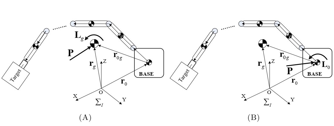
These different angular momenta give slightly different momentum equations each of which will be derived and explored in the following sub-sections.
Angular Momentum About System CoM
The total angular momentum ($L$) can be written using the angular momentum about the system CoM ($L_g$) as:
\[L = L_g + r_g \times P \ \ \ \ \ \ \ \ \ \ \ \ \ \ \ [12]\]This can be re-written as:
\[L_g = L - r_g \times P\]Here, $L$ and $P$ can be substituted from equations [9] and [10], giving the following:
\[L_g = M \tilde{r}_{g} V_0 + (\sum_{i=0}^{n} (I_i - m_i \tilde{r}_i \tilde{r}_{0i}))\omega_0 + \sum_{i=1}^{n} \sum_{j=1}^{i} (m_i \tilde{r}_i (k_j \times (r_i-p_j)) + I_ik_j)\dot{\phi}_j \\ - r_g \times (M V_0 + M \tilde{r}_{0g}^T + \sum_{i=1}^{n} \sum_{j=1}^{i} m_i (k_j \times (r_i-p_j)) \dot{\phi}_j)\]This can be simplified further as:
\[L_g = (\sum_{i=0}^{n} (I_i - m_i \tilde{r}_i \tilde{r}_{0i}) - M \tilde{r}_g \tilde{r}_{0g}^T) \omega_0 + \sum_{i=1}^{n} \sum_{j=1}^{i} (m_i \tilde{r}_{gi} (k_j \times (r_i - p_j)) + I_i k_j) \dot{\phi}_j \ \ \ \ \ \ \ \ \ \ \ \ \ \ \ [13]\]For further simplification, the following relationships are used:
\[r_g = \frac{\sum_{i=0}^{n} m_i r_i}{M},\ M \tilde{r}_g \tilde{r}_{0g} = \tilde{r}_g \sum_{i=1}^{n} m_i (\tilde{r}_i - \tilde{r_0}) = \sum_{i=1}^{n} m_i \tilde{r}_g \tilde{r}_{0i} \ \ \ \ \ \ \ \ \ \ \ \ \ \ \ [14]\]Using the above given relationships, the following equation can be derived:
\[L_g = (\sum_{i=1}^{n} (I_i + m_i \tilde{r}_{gi} \tilde{r}_{0i}) + I_0) \omega_0 + \sum_{i=1}^{n} \sum_{j=1}^{i} ( m_i \tilde{r}_{gi} (k_j \times (r_i - p_j)) + I_i k_j ) \dot{\phi}_j \ \ \ \ \ \ \ \ \ \ \ \ \ \ \ [15]\]Here, further notations can be introduced to help make the equations look more compact. Using $J_{Ti}$ and $J_{Ri}$ from before, these notations are given as:
\[H_{w} = \sum_{i=1}^{n} (I_i + m_i \tilde{r}_{gi} \tilde{r}_{0i}) + I_0 \in R^{3 \times 3}\] \[H_{w\phi} = \sum_{i=1}^{n} \sum_{j=1}^{i} ( m_i \tilde{r}_{gi} (k_j \times (r_i - p_j)) + I_i k_j ) = \sum_{i=1}^{n} (m_i \tilde{r}_{gi} J_{Ti} + I_i J_{Ri}) \in R^{3 \times n}\]Using these, the angular momentum about the system CoM can be given as:
\[L_g = H_w \omega_0 + H_{w\phi} \dot{\phi}\]Using equation [12], the total angular momentum can thus be written as:
\[L = H_w \omega_0 + H_{w\phi} \dot{\phi} + r_g \times P\]This along with the linear momentum from equation [9]:
\[P = M V_0 + M \tilde{r}_{0g}^T \omega_0 + J_{Tw} \dot{\phi}\]Can be expressed in a compact form as:
\[\begin{bmatrix} P \\ L \end{bmatrix} = \begin{bmatrix} ME & M \tilde{r}_{0g}^T \\ 0 & H_w \end{bmatrix} \begin{bmatrix} V_0 \\ \omega_0 \end{bmatrix} + \begin{bmatrix} J_{Tw} \\ H_{w \phi} \end{bmatrix} \dot{\phi} + \begin{bmatrix} 0 \\ r_g \times P \end{bmatrix} \ \ \ \ \ \ \ \ \ \ \ \ \ \ \ [16]\]The equation [16] can already be compared to equation [11] and a few differences can be observed. Firstly, the angular momentum in equation [16] does not depend directly on the linear velocity of the base-spacecraft. Instead, it depends on the Linear Momentum as seen from the last term in equation [16]. Since momentum is conserved due no lack of external forces, having a zero-initial momentum simplifies equation [16] such that the angular momentum computations are independent of the base velocity. This property is used for developing control strategies in the following works in literature: T.-C. Nguyen-Huynh, 2013 and Dimitrov and Yoshida, 2004.
Angular Momentum About Base CoM
To analyze the case of angular momentum about the base spacecraft CoM, the following equation is considered:
\[L = L_0 + r_0 \times P \ \ \ \ \ \ \ \ \ \ \ \ \ \ \ [17]\]Here, $L_0$ denotes the angular momentum about the base and $L$ the total momentum. Similar to $r_g$, $r_0$ is the vector from the inertial reference frame to the base CoM. By following a similar derivation as in the previous section, the following equation can be derived:
\[L_0 = L - r_0 \times P = M \tilde{r}_{g} V_0 + (\sum_{i=1}^{n} (I_i + m_i \tilde{r}_{0i}^T \tilde{r}_{0i}) + I_0) \omega_0 \\ + \sum_{i=1}^{n} \sum_{j=1}^{i} (m_i \tilde{r}_{0i} (k_j \times (r_i - p_j)) + I_ik_j) \dot{\phi}_j \ \ \ \ \ \ \ \ \ \ \ \ \ \ \ [18]\]Equation [18] along with the linear momentum from equation [9] can be together written in compact form as:
\[\begin{bmatrix} P \\ L \end{bmatrix} = \begin{bmatrix} ME & M \tilde{r}_{0g}^T \\ M \tilde{r}_{0g} & H_{\Omega} \end{bmatrix} \begin{bmatrix} V_0 \\ \omega_0 \end{bmatrix} + \begin{bmatrix} J_{Tw} \\ H_{\Omega \phi} \end{bmatrix} \dot{\phi} + \begin{bmatrix} 0 \\ r_g \times P \end{bmatrix} \ \ \ \ \ \ \ \ \ \ \ \ \ \ \ [19]\]Here, the $H_{\Omega}$ and $H_{\Omega \phi}$ are different from previously used $H_w$ and $H_{w \phi}$ and are described as:
\[H_{\Omega} = \sum_{i=1}^{n} (I_i + m_i \tilde{r}_{0i}^T \tilde{r}_{0i}) + I_0 \in R^{3 \times 3}\] \[H_{\Omega \phi} = \sum_{i=1}^{n} \sum_{j=1}^{i} ( m_i \tilde{r}_{0i} (k_j \times (r_i - p_j)) + I_i k_j ) = \sum_{i=1}^{n} (m_i \tilde{r}_{0i} J_{Ti} + I_i J_{Ri}) \in R^{3 \times n}\]These expressions are not always denoted by the same terms. In Yoshida et. al. 1993, $H_{\Omega}$ and $H_{\Omega \phi}$ given above are represented as $H_w$ and $H_{w \phi}$. This is in contrast with the terms used in T.-C. Nguyen-Huynh, 2013 which are also used here. In Wilde et. al. 2018, the terms $H_{\Omega}$ and $H_{\Omega \phi}$ are represented using $H_S$ and $H_{Sq}$.
Equations [16] and [19] are essentially the same equation. However, since they are both represented differently, they offer different applications. As noted in Yoshida et. al. 1993, exclusion of the $r_i$ and $r_g$ terms from the coefficient matrix of base velocities in [19] makes the coefficient matrix symmetric. Furthermore, they note that the equations [16] and [19] represent the constraints of equation of motions for the free-floating robotic system i.e the relationship between $V_0$, $\omega_0$, and $\dot{\phi}$. These equations are non-integrable about $\omega_0$ which represents a non-holonomic constraint of the system i.e this system is non-holonomic. The linear momentum part of the equations can be integrated and it can be observed that the $CoM$ of the system remains constant if the initial linear momentum is zero and remains that way i.e constant zero. However, since the angular momentum part is non-integrable, the state of the system depends on the path it takes which is a characteristic of a non-holonomic system. This results in situations which are unique to non-holonomic systems such as the free-floating robotic system in which the end-effector reaches the same initial position and orientation by following a closed loop trajectory, however the base orientation and arm configuration will not be the same.
There are other interesting differences between the equations [16] and [19] even though they represent the same system. Some of these can be seen immediately. Unlike in equation [16], in the derivation using the angular momentum about the base CoM, the angular momentum is directly linked to base linear velocity. Furthermore, the coefficient matrix of the base velocity matrix is the base inertia matrix $H_b$. This is then written as:
\[H_b = H_0 = \begin{bmatrix} ME & M \tilde{r}_{0g}^T \\ M \tilde{r}_{0g} & H_{\Omega} \end{bmatrix} \ \ \ \ \ \ \ \ \ \ \ \ \ \ \ [20]\]The base inertia matrix is also used in other equations of motion for free-floating robot manipulators as well. Furthermore, as it is an inertia matrix, it is always symmetric and invertible. The base inertia matrix is also represented as $H_0$ in Wilde et. al. 2018 and in Virgili-Llop et. al. 2016. In Wilde et. al. 2018, the equation [19] is also represented as follows:
\[\begin{bmatrix} P \\ L \end{bmatrix} = H_0 \dot{x}_0 + H_{0m} \dot{q} \ \ \ \ \ \ \ \ \ \ \ \ \ \ \ [21]\]Here, $H_0$ is the base inertia matrix as discussed before. The other terms are described as:
\[\dot{x}_0 = \begin{bmatrix} V_0 \\ \omega_0 \end{bmatrix} \in R^{6 \times 1} \ \ \ \ \ \ \ \ \ \ \ \ \ \ \ [22]\]$\dot{x}$ is the combined base velocities as shown above and $H_{0m}$ is called the dynamic coupling inertia matrix (also called base-manipulator coupling matrix in Virgili-Llop et. al. 2016) and is given below:
\[H_{0m} = \begin{bmatrix} J_{Tw} \\ H_{\Omega \phi} \end{bmatrix} \in R^{6 \times n} \ \ \ \ \ \ \ \ \ \ \ \ \ \ \ [23]\]Energy, Lagrangian, and Equations of Motion
The Lagrangian method is used to derive the equations of motion for the free-floating robot system. The potential energy of the system is taken as zero and the kinetic energy of the system can be calculated using the following set of equations:
\[L = T-V = T = \frac{1}{2} \sum_{i=0}^{n} [\omega_i^T I_i \omega_i + m_i \dot{r}_i^T \dot{r}_i] \ \ \ \ \ \ \ \ \ \ \ \ \ \ \ [23]\]Substituting equations [2] and [3] in the above equation, the following is obtained:
\[T = \frac{1}{2} \sum_{i=0}^{n} [(\omega_0 + \sum_{j=i}^{i} k_j \dot{\phi}_j)^T I_i (\omega_0 + \sum_{j=i}^{i} k_j \dot{\phi}_j) + \\ m_i (V_0 + \omega_0 \times (r_i-r_0) + \sum_{j=1}^{i} (k_j \times (r_i - p_j))\dot{\phi}_j)^T (V_0 + \omega_0 \times (r_i-r_0) + \sum_{j=1}^{i} (k_j \times (r_i - p_j))\dot{\phi}_j)]\]Expanding the terms inside the summation in the above equations gives us the following equation:
\[T = \frac{1}{2} \sum_{i=0}^{n} [ \omega_0^T I_i \omega_0 + \omega_0^T I_i \sum_{j=1}^{i}k_j \dot{\phi}_j + \sum_{j=1}^{i} \dot{\phi}_j^T k_j^T I_i \omega_0 + \sum_{j=1}^{i} \dot{\phi}_j^T k_j^T I_i k_j \dot{\phi}_j + m_i V_0^T V_0 \\ - m_i V_0^T \tilde{r}_{0i} \omega_0 + m_i V_0^T \sum_{j=1}^{i} \tilde{k}_j (r_i-p_j) \dot{\phi}_j - m_i \omega_0^T \tilde{r}_{0i}^T V_0 + m_i \omega_0^T \tilde{r}_{0i}^T \tilde{r}_{0i} \omega_0 \\ - m_i \omega_0^T \tilde{r}_{0i}^T \sum_{j=1}^{i} \tilde{k}_j (r_i-p_j) \dot{\phi}_j + m_i \sum_{j=1}^{i} \dot{\phi}_j^T (r_i^T - p_j^T) \tilde{k}_j^T V_0 - m_i \sum_{j=1}^{i} \dot{\phi}_j^T (r_i^T - p_j^T) \tilde{k}_j^T \tilde{r}_{0i} \omega_0 \\ + m_i \sum_{j=1}^{i} \dot{\phi}_j^T (r_i^T - p_j^T) \tilde{k}_j^T \tilde{k}_j (r_i-p_j) \dot{\phi}_j ]\]The terms of the above equation can be arranged based on $V_0$, $\omega_0$, and $\dot{\phi}$ and $V_0^T$, $\omega_0^T$, and $\dot{\phi}^T$ :
\[T = \frac{1}{2} \begin{bmatrix} V_0^T & \omega_0^T & \dot{\phi}^T \end{bmatrix} \begin{bmatrix} M E & M \tilde{r}_{0g}^T & J_{Tw} \\ M \tilde{r}_{0g} & H_{\Omega} & H_{\Omega \phi} \\ J_{Tw}^T & H_{\Omega \phi}^T & H_{\phi} \end{bmatrix} \begin{bmatrix} V_0 \\ \omega_0 \\ \dot{\phi} \end{bmatrix} \ \ \ \ \ \ \ \ \ \ \ \ \ \ \ [24]\]Some of the above terms have been given before, but for the sake of clarity, all the terms of the above equation are explained below:
\[J_{Ti} = \begin{bmatrix} \tilde{k}_1 (r_i - p_1) & \tilde{k}_2 (r_i - p_2) & \tilde{k}_3 (r_i - p_3) & ... & \tilde{k}_i (r_i - p_i) & 0 & 0 & ... & 0 \end{bmatrix}\] \[J_{Tw} = \sum_{i=1}^{n} \sum_{j=1}^{i} m_i (\tilde{k}_j (r_i - p_j)) = \sum_{i=1}^{n} m_i J_{Ti}\] \[J_{Ri} = \begin{bmatrix} k_1 & k_2 & k_3 & ... & k_i & 0 & 0 & ... & 0 \end{bmatrix}\] \[H_{\Omega} = \sum_{i=1}^{n} (I_i + m_i \tilde{r}_{0i}^T \tilde{r}_{0i}) + I_0 \in R^{3 \times 3}\] \[H_{\Omega \phi} = \sum_{i=1}^{n} \sum_{j=1}^{i} ( m_i \tilde{r}_{0i} (k_j \times (r_i - p_j)) + I_i k_j ) = \sum_{i=1}^{n} (m_i \tilde{r}_{0i} J_{Ti} + I_i J_{Ri}) \in R^{3 \times n}\] \[H_{\phi} = \sum_{i=1}^{n} (J_{Ri}^T I_i J_{Ri} + m_i J_{Ti}^T J_{Ti})\]Using equations [20], [22], and [23], the kinetic energy can also be written in the following forms:
\[T = \frac{1}{2} \begin{bmatrix} V_0^T & \omega_0^T & \dot{\phi}^T \end{bmatrix} \begin{bmatrix} H_0 & H_{0m} \\ H_{0m}^T & H_m \end{bmatrix} \begin{bmatrix} V_0 \\ \omega_0 \\ \dot{\phi} \end{bmatrix} \ \ \ \ \ \ \ \ \ \ \ \ \ \ \ [25]\] \[T = \frac{1}{2} \begin{bmatrix} \dot{x}_0^T & \dot{q}^T \end{bmatrix} \begin{bmatrix} H_0 & H_{0m} \\ H_{0m}^T & H_m \end{bmatrix} \begin{bmatrix} \dot{x}_0 \\ \dot{q} \end{bmatrix} \ \ \ \ \ \ \ \ \ \ \ \ \ \ \ [26]\] \[T = \frac{1}{2} \begin{bmatrix} \dot{x}_0^T & \dot{q}^T \end{bmatrix} \begin{bmatrix} H_b & H_{bm} \\ H_{bm}^T & H_m \end{bmatrix} \begin{bmatrix} \dot{x}_0 \\ \dot{q} \end{bmatrix} \ \ \ \ \ \ \ \ \ \ \ \ \ \ \ [27]\]The above methods of representation of the system kinetic energy have been used by Virgili-Llop et. al. 2016, Wilde et. al. 2018, T.-C. Nguyen-Huynh, 2013, Yoshida et. al. 1993, and K. Yoshida, 2003.
For the lagrangian, the representation from equation [26] will be taken. The generalized coordinates used to represent the system state are $[x, q]$ where $x$ is the spacecraft base position and orientation vector and $q$ is the vector containing the joint angles. Using the lagrangian ($L=T$), the equations of motion can be derived using the following Euler-Lagrange equations:
\[\frac{d}{dt} \left( \frac{\partial L}{\partial \dot{x}_0 } \right) - \frac{\partial L} {\partial x_0} = 0_{6 \times 1} \ \ \ \ \ \ \ \ \ \ \ \ \ \ \ [28]\] \[\frac{d}{dt} \left( \frac{\partial L}{\partial \dot{q} } \right) - \frac{\partial L} {\partial q} = \tau_{n \times 1} \ \ \ \ \ \ \ \ \ \ \ \ \ \ \ [29]\]The right side of equation [28] has been set to zero as this equation assumes no external forces are acting on the spacecraft base. After deriving the final equation of motion, the external forces on the spacecraft base can be added as terms on the right hand side of the equation. The right side of equation [29] constraints the vector of torques applied at the joints of the robot arm.
To continue with completing the derivation for the equations of motion, the lagrangian from equation [26] is given below:
\[L = T = \frac{1}{2} [ \dot{x}_0^T H_0 \dot{x}_0 + \dot{q}^T H_{0m}^T \dot{x}_0 + \dot{x}_0^T H_{0m} \dot{q} + \dot{q}^T H_m \dot{q} ] \ \ \ \ \ \ \ \ \ \ \ \ \ \ \ [30]\]To evaluate the partial derivatives of the lagrangian, the following matrix partial differentiation properties are used:
\[\alpha = y^T A x;\ \frac{\partial \alpha}{\partial y} = x^T A^T\] \[\alpha = x^T A x;\ \frac{\partial \alpha}{\partial x} = x^T (A^T + A)\]and if $A$ is symmetric, then:
\[\frac{\partial \alpha}{\partial x} = 2 x^T A\]Furthermore, considering the dot product between a matrix $A$ and a symmetric matrix $B=B^T$, the following relations are used as inertia tensors are symmetric by definition:
\[A^T B = A \cdot B = B \cdot A = B^T A = B A\]Using the above given relations, the partial derivative of the lagrangian given in equation [30] is evaluated with respect to the generalized coordinates:
\[\frac{\partial L}{\partial \dot{x}_0} = \frac{1}{2} [ 2 \dot{x}_0^T H_0 + \dot{q}^T H_{0m}^T + \dot{q}^T H_{0m}^T ] = \dot{x}^T H_0 + \dot{q}^T H_{0m} = H_0 \dot{x}_0 + H_{0m} \dot{q} \ \ \ \ \ \ \ \ \ \ \ \ \ \ \ [31]\] \[\frac{\partial L}{\partial \dot{q}} = \frac{1}{2} [ \dot{x}_0^T H_{0m} + \dot{x}_0^T H_{0m} + 2 \dot{q}^T H_m] = \dot{x}_0^T H_{0m} + \dot{q}^T H_m = H_{0m}^T \dot{x}_0 + H_m \dot{q} \ \ \ \ \ \ \ \ \ \ \ \ \ \ \ [32]\]Evaluating the derivate of the above given equations with respect to time can be given as:
\[\frac{d}{dt} \left( \frac{\partial L}{\partial \dot{x}_0 } \right) = H_0 \ddot{x}_0 + \dot{H}_0 \dot{x}_0 + H_{0m} \ddot{q} + \dot{H}_{0m} \dot{q} \ \ \ \ \ \ \ \ \ \ \ \ \ \ \ [33]\] \[\frac{d}{dt} \left( \frac{\partial L}{\partial \dot{q} } \right) = H_{0m}^T \ddot{x}_0 + \dot{H}_{0m}^T \dot{x}_0 + H_m \ddot{q} + \dot{H}_m \dot{q} \ \ \ \ \ \ \ \ \ \ \ \ \ \ \ [34]\]The equations [33] and [34] represent the first terms of the equations [28] and [29]. The second terms of the equations [28] and [29] can be written as (from Wilde et. al. 2018):
\[c_0 = - \frac{\partial L} {\partial x_0} = \frac{1}{2} \frac{\partial}{\partial x_0} \left( \dot{x}_0^T H_0 \dot{x}_0 + \dot{q}^T H_{0m}^T \dot{x}_0 + \dot{x}_0^T H_{0m} \dot{q} + \dot{q}^T H_m \dot{q} \right) \ \ \ \ \ \ \ \ \ \ \ \ \ \ \ [35]\] \[c_m = - \frac{\partial L} {\partial q} = \frac{1}{2} \frac{\partial}{\partial q} \left( \dot{x}_0^T H_0 \dot{x}_0 + \dot{q}^T H_{0m}^T \dot{x}_0 + \dot{x}_0^T H_{0m} \dot{q} + \dot{q}^T H_m \dot{q} \right) \ \ \ \ \ \ \ \ \ \ \ \ \ \ \ [36]\]Using the equations [28]-[29] and [33]-[36], the equations of motion can be written as:
\[\begin{bmatrix} H_0 & H_{0m} \\ H_{0m}^T & H_m \end{bmatrix} \begin{bmatrix} \ddot{x}_0 \\ \ddot{q} \end{bmatrix} + \begin{bmatrix} \dot{H}_0 & \dot{H}_{0m} \\ \dot{H}_{0m}^T & \dot{H}_m \end{bmatrix} \begin{bmatrix} \dot{x}_0 \\ \dot{q} \end{bmatrix} + \begin{bmatrix} c_0 \\ c_m \end{bmatrix} = \begin{bmatrix} 0_{6 \times 1} \\ \tau_{n \times 1} \end{bmatrix} \ \ \ \ \ \ \ \ \ \ \ \ \ \ \ [37]\]This representation of equation of motion for a robot manipulator with free-floating base is given in Wilde et. al. 2018.
In most literature (such as in Virgili-Llop et. al. 2016, K. Yoshida, 2003, and K. Yoshida & B. Wilcox, 2008), the non-linear velocity dependent terms are coupled together in one term (as done in the generalized manipulator equation in robotics, equation 4.24 in Murray et. al. 2017) and written as $\begin{bmatrix} c_b & c_m \end{bmatrix} ^T$. Thus, the equation can be written in a compact form as:
\[\begin{bmatrix} H_0 & H_{0m} \\ H_{0m}^T & H_m \end{bmatrix} \begin{bmatrix} \ddot{x}_0 \\ \ddot{q} \end{bmatrix} + \begin{bmatrix} c_b \\ c_m \end{bmatrix} = \begin{bmatrix} 0_{6 \times 1} \\ \tau_{n \times 1} \end{bmatrix} \ \ \ \ \ \ \ \ \ \ \ \ \ \ \ [38]\]In the above equation [38], the forces and torques acting on the center of mass of the base can be added to the right-hand side as a force-torque ( $F_b \in R^{6 \times 1}$ ) vector inside the matrix and written as follows:
\[\begin{bmatrix} H_0 & H_{0m} \\ H_{0m}^T & H_m \end{bmatrix} \begin{bmatrix} \ddot{x}_0 \\ \ddot{q} \end{bmatrix} + \begin{bmatrix} c_b \\ c_m \end{bmatrix} = \begin{bmatrix} F_{b} \\ \tau_{n \times 1} \end{bmatrix} \ \ \ \ \ \ \ \ \ \ \ \ \ \ \ [39]\]This method of using generalized coordinates and writing equations of motion for a manipulator is prevalent in the robotics literature. A very common compact form of writing the equations [37], [38], and [39], can be taken from Choset et. al. 2005 and written as:
\[M(q)\ddot{q} + C(q, \dot{q})\dot{q} = \tau \ \ \ \ \ \ \ \ \ \ \ \ \ \ \ [40]\]Here, $\tau$ represents the generalized forced applied to the system as given in equation [39]. However, in the scope of earth-based robot systems, the $\tau$ is usually written with a subscript $\tau_g$ to represent the generalized forces due to gravity. Equation [40] can further be extended to add other generalized forces applied to the system and written as:
\[M(q)\ddot{q} + C(q, \dot{q})\dot{q} = \tau_g(q) + B(q)u + J^T F_c + F_f \ \ \ \ \ \ \ \ \ \ \ \ \ \ \ [41]\]Here the terms given are:
$q$ - Generalized Coordinates of the System
$M(q)$ - Mass-Inertia Matrix of the System
$C(q, \dot{q})$ - Coriolis Force Terms
$\tau_g(q)$ - Generalized Forced due to Gravity
$B(q)$ - Matrix to Map the Control inputs to generalized forces
$u$ - Control Inputs
$J$ - Jacobian to Map the Contact Forces to Generalized Forces
$F_c$ - Contact Forces
$F_f$ - Generalized Friction Forces
Equation [41] represents the complete dynamics of a multibody system. The equation can be thought of as the $ma=F$ equation for easier understanding. However, not all terms in the equation represent a force directly. From Choset et. al. 2005: The equations of motion given in [41] depend on the choice of coordinates $q$. For this reason neither $M(q)\ddot{q}$ nor $C(q, \dot{q})\dot{q}$ individually should be thought of a generalized force; only their sum is a force.
Linearized Equations of Motion
The chapter on linearized form of the equations of motion for a free-floating multibody system can be found here.
References
[T.-C. Nguyen-Huynh 2013] T.-C. Nguyen-Huynh, “Adaptive Reactionless Control of a Space Manipulator for Post-Capture of an Uncooperative Tumbling Target,” McGill University, 2013.
[Wilde et. al. 2018] M. Wilde, S. K. Choon, A. Grompone, and M. Romano, “Equations of motion of free-floating spacecraft-manipulator systems: An Engineer’s tutorial,” Front. Robot. AI, vol. 5, no. APR, pp. 1–24, 2018.
[Yoshida et. al. 1993] K. Yoshida and Y. Umetani, “Control of Space Manipulators with Generalized Jacobian Matrix,” 1993, pp. 165–204.
[Dimitrov and Yoshida, 2004] D. N. Dimitrov and K. Yoshida, “Momentum distribution in a space manipulator for facilitating the post-impact control,” 2004 IEEE/RSJ Int. Conf. Intell. Robot. Syst., vol. 4, pp. 3345–3350, 2004.
[Virgili-Llop et. al. 2016] J. V. Virgili-Llop, D. Drew, and M. Romano, “SPACECRAFT ROBOTICS TOOLKIT : AN OPEN-SOURCE SIMULATOR FOR SPACECRAFT ROBOTIC ARM DYNAMIC MODELING AND CONTROL . Josep Virgili-Llop , Jerry V . Drew II , Marcello Romano Spacecraft Robotics Laboratory Naval Postgraduate School Monterey CA USA,” 6th International Conference on Astrodynamics Tools and Techniques. 2016.
[K. Yoshida, 2003] K. Yoshida, “Engineering test satellite VII flight experiments for space robot dynamics and control: Theories on laboratory test beds ten years ago, now in orbit,” Int. J. Rob. Res., vol. 22, no. 5, pp. 321–335, 2003.
[K. Yoshida & B. Wilcox, 2008] K. Yoshida and B. Wilcox, “Space Robots and System,” in Springer Handbook of Robotics, no. November 2015, 2008.
[Murray et. al. 2017] R. M. Murray, Z. Li, and S. Shankar Sastry, A mathematical introduction to robotic manipulation. 2017.
[Choset et. al. 2005] H. Choset, K. M. Lynch, S. Hutchinson, G. Kantor, W. Burgard, L. E. Kavraki, and S. Thrun. Principles of Robot Motion-Theory, Algorithms, and Implementations. The MIT Press, 2005.