Space Rendezvous/ Formation Flying/ (Autonomous) Close Proximity Navigation
Technological importance
Space rendezvous maneuvers are relevant for several types of space activities, such as
- Resupply of orbital structures like the International Space Station (ISS)
- Assembly of large structures like the ISS
- Sample return missions like the Hayabusa2 of JAXA
- Spacecraft servicing or repair missions such as the Hubble Servicing Missions
- Active debris removal missions
Previous missions
Successful rendezvous maneuvers have been demonstrated in quite a few missions in the past already.
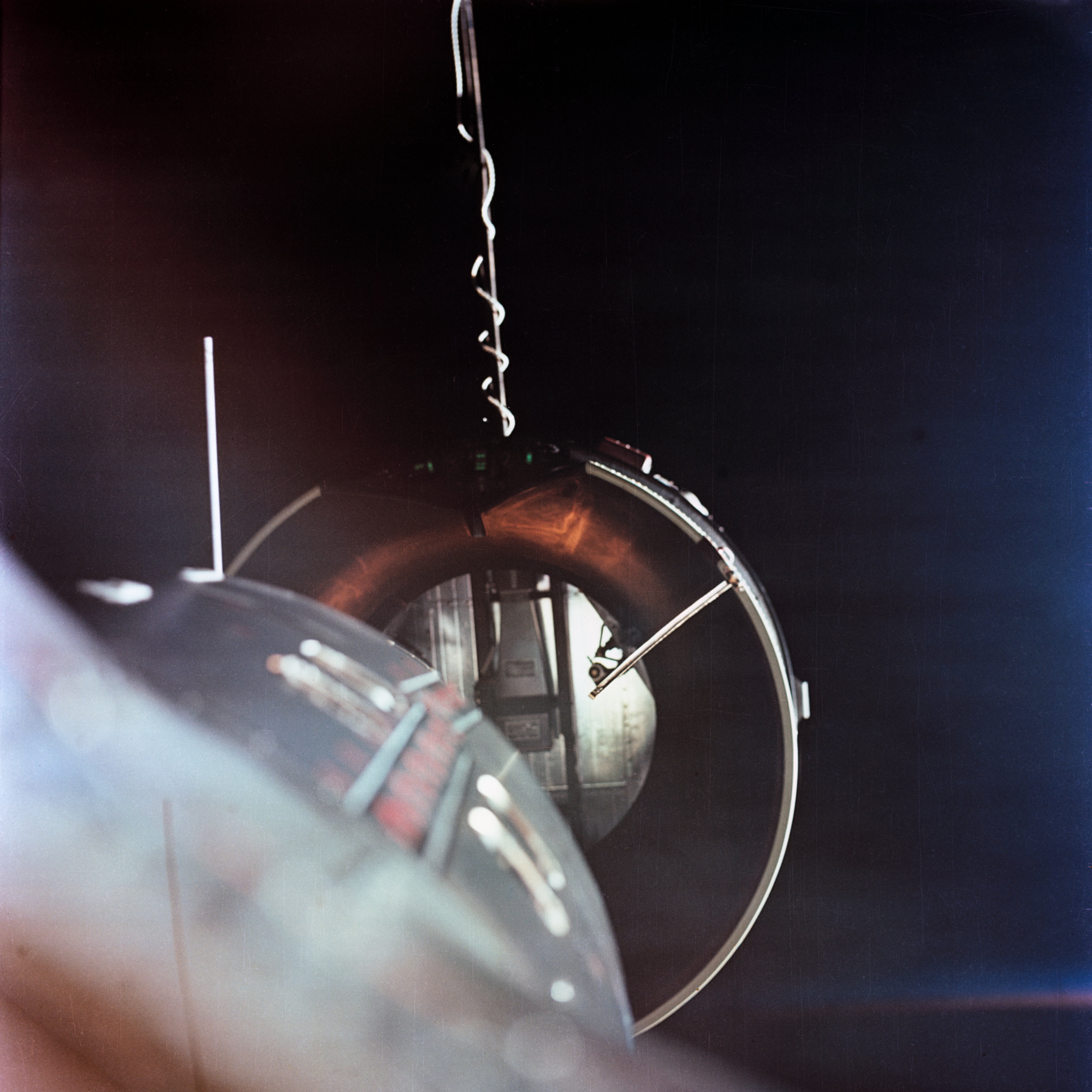
In 1966, Gemini 8 docked with Agena - the first recorded space docking maneuver. The docking itself was a success, but there was a problem with the attitude control systems after docking, which threatened the lives of the astronauts via an accelerating rotation of the combined spacecraft. The astronauts undocked the spacecraft, and were able to, via some very lucid trouble-shooting, to stop the dangerous rotation.
The docking of Gemini 8 and Agena was a manually conducted maneuver. The first automated rendezvous maneuver was conducted between the two Soviet Union spacecraft Kosmos 186 and Kosmos 188. Mechanically, the docking was a success, though establishing an electrical connection failed. The Soviet Union was motivated to pursue the development of automated docking technology due to the fact that they had no ground stations outside of their own territory.
_drawing.png)
Since these first rendezvous mission, there have been many more. In most of these missions involving docking, astronauts have been involved. Automatic rendezvous is becoming more relevant due to the increased presence of mankind in space and the fact that all of our planned activities cannot be directed from ground. The preferred, safer kind of automatic rendezvous is cooperative, such that the target vehicle might provide navigation aids and/or stabilizes its own attitude for the vehicle about to dock. However, the need to counter the onset of the Kessler syndrome and to study small bodies in space forces interaction with uncooperative objects. These types of missions require the approaching spacecraft to do all the work regarding sensing, computation, and movement.
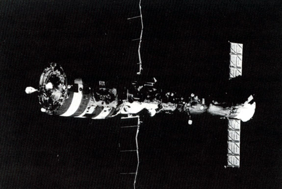
The first docking to a dead satellite occurred in 1985, when the Soyuz T-13 mission performed a manned manual docking to the dead Salyut 7 space station, which had experienced a failure of the solar power system. Mechanical levers were added to the Soyuz spacecraft for proximity operations. The crew used a handheld laser rangefinder to measure distance to the target. The Soyuz crew piloted the spacecraft to match the rotation of the target before finally docking. The repair operations that followed returned to Salyut 7 to an operational state, stabilizing its attitude. Due to this, normal resupply missions with Progress supply spacecraft could resume.
The missing pieces
The technology to automatically rendezvous with an uncooperative targets in space is not mature as of writing this at the end of 2019. To start with, it is not clear which sensors have the greatest potential to perform the automated rendezvous successfully. For most of the traditional sensors like cameras and lidar there has been a significant amount of work regarding sensor data processing in order to extract quickly and precisely data about the relative position and orientation of the target spacecraft. One can imagine that extracting the exact position and orientation of a target spacecraft from a flat grayscale image, for example, requires fairly heavy calculations. Unfortunately, all of the solutions so far demonstrate some sort of vulnerabilties or limitations that can yield incorrect relative states of the target in certain conditions. Due to this there is still a need for further research regarding additional processing to interpret the correctness of the result. There is a need to understand when a failure has occurred and the output of the calculations is an incorrect relative position or orientation. In addition, there need to be reliable methods of recovering from a failure of these algorithms. There are of course operational limits to these algorithms that need to be well understood. For example, let’s assume we have chosen a visible light camera and we have a digital model of the spacecraft, which allows us to compare the images we take to the model in order to determine the relative positition and orientation of the target. How accurate does that model need to be? Does it have texture? What if the spacecraft is damaged and has a significant visual deviation from the model we have? As we can see, there are still plenty of questions to be answered.
Mission profile and specific issues of close range rendezvous and physical interaction with targets
A typical rendezvous and docking mission can be distinctly divided into several phases.
- Launch: the chaser spacecraft (the one that is about to pursue docking with another satellite already in orbit) is injected into the orbital plane of the target and its orbital conditions are stabilized.
- Phasing: the phase angle or the angular distance between the chaser and target is reduced using absolute navigation sensors, like GPS, for example. In general the altitude of the chaser is lower than that of the target, since the faster orbit velocity naturally carries the chaser closer to the target.
- Far range rendezvous: the start of this phase marks the beginning of relative navigation as a means of closing in further with the target. The switch is made as absolute navigation is lacks the accuracy of closing in further safely. The starting location of this phase depends on the location of the physical features on the target that will be interacted with as a part of the capture operations.
- Close range rendezvous: here the objectives are to close the last bit of distance to the target such that the target is in range for capture, whatever the chosen mechanism for that is. Furthermore, part of this phase is to align the chaser with the final approach axis such that the chaser approaches directly toward the interfaceable component on the target. For example, this could be a thruster nozzle for an upper stage or a launcher adapter ring for a payload.
- Mating: this refers to establishing a structural connection with the target. There are many options for this, like nets, harpoons, robotic arms, clampers, etc. To read more about robotic-arm capture systems, please refer to the page on Space Robotics: On-Orbit Servicing and Debris Removal.
The navigation requirements are strictest in the last two phases of close range rendezvous and mating, as the risk of collision increases. Often these navigation requirements dictate the addition of sensors that were not needed in previous phases. The chaser needs to know the target’s relative position, velocity, rotation, and rotation rate in order to be able to match a possible tumbling and be able to target the capture mechanism. If a net enveloping the target is used, these requirements are not so strict. If a robotic arm is used, however, the tool tip has to align fairly accurately with a specific position on the target.
Close range rendezvous and mating also tend to involve non-natural trajectories where propulsion has to be employed in order to achieve a certain trajectory. In this sense it is desirable for the close range navigation system to be performant enough such that this motion forcing does not take more time than necessary for reducing requirements on the propulsion system.
It is very expensive and difficult to ensure contact with the chaser from the ground at all times during the final phases of a rendezvous and mating mission. What is more, ground based control of the approach is also difficult and unsafe. Therefore, it is very desirable that the chaser is able to autonomously navigate and make safe decisions.
Sensors and relative states of target spacecraft
Several types of sensors have been considered for the purpose of exctracting relative position and attitude of an uncooperative target:
- Pulse and continous-wave laser rangefinders: there are many subtypes of sensors in this category, but the suitable ones capture information about a field of view wide enough to measure the whole target during close range approach and possibly mating. The resolution of the measurements also has to be fine enough to discern target attitude and position from the measurements.
- Camera-type sensors: this category also has subtypes of sensors, mostly to do with different wavelengths of light being measured. The main idea is that a detector captures an image at the focal plane of a lens. Here as well the camera has to have a high enough resolution that the landmark features on the target that are used for relative navigation are actually discernible.
This is not an exhaustive list as new sensor types are appearing, particularly in the field of earthbound robotics. For example - optical flow and event cameras. For the purposes of keeping an open mind for research, the selected sensor has to discern features on the target such that its position and attitude are implied in the sensor data. Furthermore, it was to withstand the space environment and also not have any showstopping disadvantages. For example, the lighting conditions in space can be very challenging with parts of the spacecraft reflecting so much light that they appear saturated on the image while other shadowed parts are barely visible. This can interfere with laser and camera measurements and also the interpretation of those measurements. Many of the algorithms interpreting sensor data for extraction of relative attitude and position include characteristics meant to overcome these poor lighting conditions and also, for example, seeing the Earth in the background.
The requirements of knowing the target’s position and rotation (in literature referred to as the 6-dimensional object pose estimation problem) is surprisingly demanding in terms of computational power. That is because the information about these states in any of the available sensors’ data is implicit. As an example, a camera’s flat image of a target spacecraft offers only pixels describing light intensity - there is no explicit information about how the target is rotated or positioned. Given a toy model of the target spacecraft, a human can try to visually match what he or she sees on the image by moving the toy further away from the eye to reduce the optical size and also rotate it somehow along all axes such that the same parts and sides of the spacecraft are similarly visible. Herein lies the challenge - what mathematics can be employed to do that automatically, more precisely, faster, and more reliably than a human? This also applies to other sensors besides cameras. Given a point cloud from a flash lidar sensor, how does one interpret it as a relative position and orientation of the target?
There are already plenty of solutions that do this to some degree. A popular approach is to extract edges from an image of the target that then can be compared to a wireframe model of the target spacecraft. One does not have to be limited to edges - corners, textures, and other features can also be used as a comparison between an image and a model. Features can also be learned via neural networks, for example. Of course there are approaches beyond those using local descriptors such as edges and the approaches differ wildly in architecture and computation. The important thing is that none of them are infallible. All of them lack in robustness which will have to be compensated via failure detection and recovery methods in order to achieve a design reliable enough for autonomous rendezvous and capture. Due to the large variety of approaches there are also a large variety of methods to increase robustness, though some themes are common. One could, for example, use knowledge of the dynamics of the target or previous image to enforce a reasonable continuity of the relative states of the target. There are also additional problems to consider such as symmetric targets, targets that differ significantly from available models of them, targets that lack a model entirely, targets lacking the features necessary for the pose estimation algorithm, the specific problems of the mathematics (predictability or domain adaptation of learning algorithms such as ones using neural networks), and also applicable ranges to target.
Verification & Validation
Proximity navigation solutions can be validated in a number of ways:
- Simulations: are meaningful for functional and software testing, but are limited to a certain degree of realism that might only coarsely hint at the true performance of the solution.
- Hardware-In-The-Loop: simulations involving hardware to some extent can reflect hardware-specific issues and might provide further realism in terms of a real environment and offer real-time simulation capability. Often the simulatable scenarios tend to be limited.
- In-orbit validation: the most expensive, but most realistic measure of performance of a solution.
Introduction to object pose estimation
Object pose estimation is an integral part of close-range visual relative navigation with uncooperative targets. It is relevant for future activities such as on-orbit servicing and active space debris removal. Generally, two tasks can be distinguished in pose estimation systems - initialization and tracking. Initialization refers to a situation with no previous information about where a sought target is in the sensor field of view. Tracking refers to a situation where previous estimates are available (after initialization) and so the search space for an estimate is smaller. Technology demonstrations so far have handled these tasks via solutions like template matching or image processing algorithms, perhaps seeking to fit lines of a wireframe model to the lines found in the image, for example. See [Sharma et al., 2016] for a comparison of pose initialization techniques that are not based on convolutional neural networks. The general computer vision field has focused on convolutional networks instead, also for navigational tasks. Bringing convolutional neural networks over to visual relative navigation in space would potentially offer several advantages over the state of the art. To start with, they could be flexible towards all kinds of target objects, not just ones that have distinguishable lines or silhouettes. Furthermore, they can learn whatever visual features are useful for the performance of the task, not just manually designed visual features like lines. If this flexibility can be capitalized on, CNNs could form a basis for a general visual relative navigation system that does not require a new integration for every new target with a possibly different appearance.
Object pose estimation using CNNs
This section reviews the state of the art for estimation of spacecraft pose from images with convolutional neural networks. In the context of relative navigation with spacecraft, “pose estimation system” as a term can refer to a combined assembly of multiple distinct subsystems. It is not uncommon to obtain an initial pose estimation via a “pose initialization” subsystem. This is usually an image processing algorithm that takes a camera image as an input and outputs the very first pose estimate without having access to a prior estimate, which means the search space for an estimate is the largest at this point in the comprehensive pose estimation system. Once this is achieved, it is also normal to encounter a “pose tracking” subsystem following the pose initialization. This could be a plain state estimator like a Kalman filter or a visual tracker or both combined.
A review of spacecraft pose estimation using CNNs
The Stanford Rendezvous Laboratory (SLAB) has made a sizeable contribution to the task of estimating pose from images with CNNs. In 2018, Sharma et al made the first step at SLAB to apply convolutional neural networks to the task of spacecraft pose estimation from images [Sharma et al., 2018]. The paper documents two primary contributions - the first is a convolutional neural network intended for pose initialization. The network is set up to fit a classification task, so the output of the last layer is used in a softmax loss function, which produces a distribution over the class labels. The classes are tied to a discretization of the pose space such that each class refers to a particular pose estimate (a single rotation matrix, for example). During training, the closest discrete estimate is chosen as the ground truth for the training images. The second major contribution of the paper is the development of a synthetic image generation pipeline to train the neural network. The pipeline is intended to produce an abundance of images that represent noise, color, and illumination characteristics expected in orbit. The European Space Agency (ESA) and SLAB partnered to organize a Pose Estimation Challenge on the Kelvins platform, where competing pose estimation systems were benchmarked on the SPEED dataset [Kisantal et al., 2020]. The post-competition analysis of Kisantal et al. found that all 20 submissions used deep learning as a part of their pose estimation pipeline.
Compatibility of symmetric target objects and CNN-based pose estimators
Given a target object that exhibits symmetry, one can run into the issue of pose ambiguity. This is a condition where the object seen on the image could possibly correspond to multiple or even an infinite number of unique pose estimates. It is difficult to describe the orientation of a textureless perfect sphere, for example. Consider a difficult case in the space environment - it is very easy to run into cylindrical objects, in which case it might also be difficult to describe its orientation about the rotational axis. It is desirable to have a navigation system that does not have to be changed drastically depending on the target object, therefore it is a good idea to design for symmetrical objects from the beginning. Additionally, it is worth noting that this condition of ambiguity can also occur when the local details on the physical spacecraft that are attributable to a certain pose are obscured by a shadow or an intense reflection of the Sun, for example. This section gives an overview of how symmetry has been dealt with in the context of using convolutional neural networks for pose estimation. Finally, works dealing with spacecraft pose estimation using convolutional neural networks are analyzed from the perspective of being prepared to handle symmetric objects.
CNN-based pose estimation work has arrived at many different ways to adapt to symmetric targets. This is partially due to the many ways that CNNs can be used to arrive at a pose estimate.
Kehl et al. [Kehl et al., 2017] use a viewpoint classifier to obtain a pose estimate. Viewpoint classifiers are able to tolerate better a one-to-many type problem as arises with viewpoint ambiguity, but still there are convergence problems. To circumvent these, the authors select a subset of viewpoints during training such that ambiguous redundant poses are removed. This still requires manual intervention for every new type of object.
Rad et al. [Rad et al., 2017] solve this issue for a keypoint-regressing network by restricting the keypoint labels to a pose interval where no ambiguity is present. The absolute pose is then obtained by a separate classifier that tries to determine which of the ambiguous pose intervals is present (if at all distinguishable) and this is taken into account in the final pose estimate. This process is not preferable as the intervals are manually designed and every new target would require a new consideration. Furthermore, this does not work for objects with infinite ambiguous viewpoints such as a cylinder.
Corona et al. [Corona et al., 2018] also use an embedding via a a convolutional neural network and then selecting the closest latent vector from a dictionary of discrete viewpoints as the final pose estimate using cosine similarity. However, they additionally classify the order of the symmetry with a classifier. This symmetry classification still requires manual intervention to label symmetry orders for the target object.
Xiang et al. [Xiang et al., 2018] approach symmetric objects by using a loss function that focuses on the closest vertices of the 3d model of the object being in agreement between estimate and ground truth orientations. A perfect application of this logic would also assume a symmetric mesh for the object, which is not always the case. Furthermore, this approach comes with local minimums.
Sundermeyer et al. [Sundermeyer et al., 2018] presents a methods for estimating the pose of an object with convolutional neural networks that uses the convolutional network to encode an image into a latent space vector. This vector then is used as a key to a dictionary using cosine similarity, yielding a pose estimate. The dictionary is inherently able to handle ambiguous poses as there is no conflict between storing very similar vectors being stored as keys.
Park et al. [Park et al., 2019] uses a principle they call ‘transformer loss’ to train their network to estimate the pose of a symmetric target. Essentially, the keypoints of the closest plausible ambiguous pose to the predictions of the network are chosen for each image in a training batch.
Manhardt et al. [Manhardt et al., 2019] propose a fairly general method where a high number of redundant poses are predicted for an object. Due to the high number of redundancy, the output is expected to reflect a distribution of poses that are plausible given a particular input image. However, the suitability of this approach depends on the output of the neural network. This approach works quite well if the output of the neural network is a rotation representation directly, such as a quaternion. However, many modern pose estimation frameworks actually estimate 2D image space keypoints, which are then resolved to a pose via a Perspective-n-Point solver. This is done, because keypoints are easier to regress than quaternions, for example. However, Manhardt’s approach gets complicated when a set of keypoints are estimated. The process gets more intensive as more keypoints are used, and then there is the difficulty of having to move from 2D image space to pose space with all these reduntant keypoint regressions.
Hodan et al. [Hodan et al., 2020] present a new approach to the pose estimation of symmetric objects. Essentially, a neural network is used to segment the surface of the target object in the image into patches. To reiterate, the surface of the target object is divided into some fragments of the whole, and these are then classified in the image per pixel. Per each identified fragment, a regressor is used to estimate the 3D coordinate of the fragment’s center. These 2D-to-3D correspondences are then used with the Progressive-X scheme incorporating a robust and efficient PnP-RANSAC algorithm. In addition to inherently dealing with symmetric objects, this approach has the added value of not needing specific features on the object to relate keypoints to, which has been a problem for landmark-regressing or bounding-box-corner-regressing approaches.
Rathinam et al. [Rathinam et al., 2020] compare a viewpoint classifider and an architecture that features an object detector for initial image cropping, a keypoint regressor, and a PnP-solver. They note that to achieve similar results, the viewpoint classifier requires approximately 6-10 times more trainable parameters. However, they do stress that this depends heavily on the setup of the system. Furthermore, this does not take into account the PnP-solver that is still necessary to move from keypoints to an actual pose.
It’s interesting to a look at how existing pose estimation systems applied to spacecraft have tackled the issue of symmetry.
From the perspective of symmetric target objects, the neural network of Sharma et al from [Sharma et al., 2018] is suitable for symmetric objects, in the sense that images containing ambiguous viewpoints will yield some class probabilities that reflect uncertainty between the plausible pose estimates. Of course, the issue remains then that one of these ambiguous solutions will have to be chosen as an initial pose estimate for downstream systems that rely on it. This could be a Kalman filter, for example. Essentially, the ambiguity is passed downstream from the neural network. If this pose estimate would be naively connected to a state estimator, it would seriously disturb the accuracy of the state estimate every time the pose initializer jumps to an alternative plausible pose estimate.
Target image scale variation in pose estimation
Another issue that one often runs into as a result of viewing objects at various distances is that neural networks have to learn relationships at different scales. In the context of pose estimation, often this is overcome by using a separate neural network inference run to crop the object in the image, because moving on to the actual pose estimation task. It is desirable to reduce the number of required components and learned parameters, so research has been done to adapt existing methods to interpreting objects at various ranges.
Cheng et al. [Cheng et al., 2020] apply a neural network to the task of human pose estimation using a couple of modications to improve the scale-difference learning. Namely, they supervise the training at multiple scales in the network as well as aggregating layers at multiple scales for inference.
Domain-related robustness of demonstrated CNN-based pose estimators
CNNs are commonly justified in image processing applications due to their flexibility in terms of learned features and objects, as well as a robustness to viewing conditions. However, these aspects are not guaranteed. It’s easy to set up a training dataset such that the neural network learns some pattern during training that is not available in realistic conditions. Or, perhaps not enough visual variety was introduced in the training dataset to enable the network to operate in different lighting conditions. This section reviews the methods that reviewed CNN-based pose estimation systems have used to leverage these advantages. Sharma et al in their first generation CNN-based pose estimation system [Sharma et al., 2018] do not really explore the robustness of the trained network. The test dataset is independent from training and validation datasets, but they are sampled from the same domain. Therefore there is no evaluation of how the performance of the network would change in different viewing conditions - it’s not evaluated on real images or even synthetic images with significantly different lighting strength.
Segmentation-based pose estimation
Segmentation-based pose estimation is a technique recently introduced to the task of pose estimation [Hu et al., 2019]. Gerard et al. [Gerard 2019] used the CNN featured in this work in the ESA Kelvins Pose Estimation Challenge to rank second in the leaderboard, with the highest score on real images. In the case of visual-sensor-based spacecraft pose estimation, the desirable workflow for applying an image processing neural network is to train it on synthetic images and apply it on real images when deployed in its final application. Therefore this particular pose estimation technique stands out from the Kelvins Pose Estimation Challenge. It has recently been applied again to spacecraft pose estimation on a different, symmetric target [Kajak et al., 2021]. Furthermore, many more real camera images were used to evaluate the neural network. Additionally, in one evaluation case zero real camera images were used during training, while the network was shown to work on real camera images from a different domain, thanks to the application of domain randomization. The following sections explain how that was achieved.
Modifications to cope with symmetric objects
The segmentation-based pose estimation system of and its training procedure as presented by Hu et al. [Hu et al., 2019] is not prepared to cope with symmetric targets as is. Not being prepared to handle symmetric objects easily is quite a limitation as many man-made objects in space are symmetrical. For example, upper stages that are responsible for a substantial amount of fragmented space debris are an excellent active debris removal target [Opiela 2009] from the perspective of mitigating debris collision risk. They are, however, nearly symmetrical. A fairly recent work by Park et al. [Park et al., 2019] uses a training loss that adjusts the pose label to the nearest symmetry-aware plausible pose such as to pull the estimates of the network toward one of the ambiguous poses. This approach is adopted in this work also as well as a modified variation. It’s a preferred solution as it is a simple change to get the network presented by Hu at al. to perform with symmetric objects.
Production of synthetic camera images of spacecraft in relative navigation setting using Blender
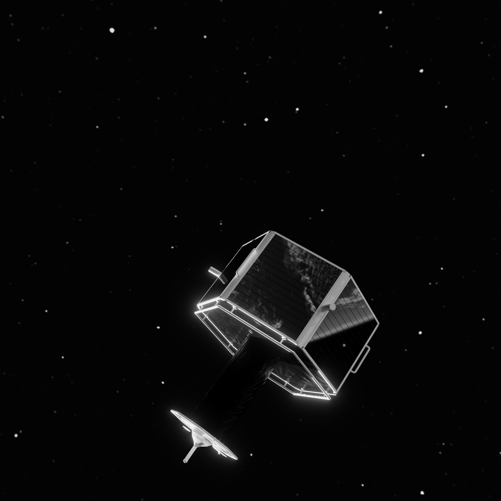
The open-source 3D-rendering software Blender is used to generate simulated synthetic images of a representative target spacecraft in relative navigation scenarios, as if a chaser spacecraft were observing it. A few sample images are shown in Figure 1. The following subsections describe detailed aspects of the rendering settings. The render itself is discussed, as well as the scene and its components. The scene is composed of a spacecraft, a background, and light sources.
Rendering engine
The renderer used to generate the synthetic images is a raytracing engine called Cycles. The use of a raytracer allows the generation of more realistic shadows and reflections, which are important in relative navigation settings. Often the only source of light in the orbital environment is the Sun and therefore significant parts of the spacecraft can be obscured by shadows. Furthermore, there can be a very large brightness difference between lit and unlit areas of the spacecraft. Also, many spacecraft incorporate highly reflective materials and components such as solar panels or Multi-Layer Insulation (MLI). The intention is not so much to have the most accurate reflections possible, but rather to have a similar type and level of variability associated with the appearance of the reflective parts of the spacecraft. Furthermore, the raytracer is able to mimic under-/overlighting situations fairly realistically. Not relying on heavily shadowed areas is something the neural network should be able to do, ideally. The same goes for heavily overlit areas. The environment has to feature something to reflect off of the spacecraft, though, to uphold this logic.
Background environment
The background of the rendered environment is varied in the synthetic images used to train the neural networks. The baseline background is a panoramic image taken at an Earth orbit position, produced using SpaceEngine. It is an HDR-image, so the stars and Sun are visible simultaneously. This is perhaps not realistic, but it adds more visuals to reflect off of the MLI and the solar panels. The particular height of the orbital position or the lighting environment does not matter too much as the background is merely added to provide somewhat realistic reflections for training. The orientation of the background is randomized along all three axes. The datasets used in the section “Domain randomization for sim2real and robustness” feature modifications to this background baseline. The first modification is that the brightness of the background is allowed to vary between fairly bright and entirely black. The second modification is that Blender’s procedural textures ‘Magic’ and ‘Voronoi’ are also mixed in with the original space environment image at randomly varying strengths. The reasoning behind these modifications is explained further in section “Domain randomization for sim2real and robustness”, but briefly stated this is to prevent the neural network to get used to a specific background and level of contrast between the spacecraft and background.
Lighting and camera sensor
There is a “Sun” light source in the scene besides the background, which also emits light, emulating an Earth albedo component. The “Sun” light source is a parallel ray light source to mimic the real Sun. For the datasets in section “The problem of a symmetric spacecraft target” merely the direction of the Sun is randomized. For the datasets in section “Domain randomization for sim2real and robustness” the Sun’s light emission strength is also varied between a bright value and nearly completely dark value. Furthermore, the camera exposure time is varied in order to provide globally dark or bright images as well.
Spacecraft
The digital 3D-model of the spacecraft is a simplified version of a physical mockup described in section “Pseudo-real images of physical spacecraft mockups in relative navigation setting and EPOS 2.0 laboratory”. It exhibits finite symmetry about its longitudinal or docking axis, though at various multiplicities. There are three material groups used in the model. The front hexagonal plate and column are wrapped in MLI, which is mimicked via a golden reflective material. The folds of the MLI are replicated via Blender’s procedural ‘Voronoi’ and ‘Magic’ textures applied to the surface normal map, which means that light bounces off the surface chaotically, just as it would off a folded and crinkled foil. The second material is the solar panel, mounted on the sides of the hexagonal main body of the spacecraft. This is also a reflective material with a dark blue hue. The third material is a glossy white paint featured on the details of the body and docking adapter. The model is simplified in the sense that it lacks certain MLI cutouts that are featured on the physical mockup as well as some small scale details like screws that are a part of the original complex CAD drawing of the spacecraft. There are a few further discrepancies. One of them is a missing solar panel plate on one side of the hexagonal body, which leaves a gap where one can look at the interior of the physical mockup. The second discrepancy is that the front hexagonal railing on the docking adapter has been deformed slightly (a few centimeters out of the plane of the railing) due to impacting the floor in a previous accident. Overall, these differences should not stand in the way of applying a network trained with simulated images on real images of the physical mockup taken with a camera. They are rather viewed as opportunities to see how local differences impact tested neural network solutions. The above-described setup is used for datasets in section “The problem of a symmetric spacecraft target” for training and testing. The datasets in section “Domain randomization for sim2real and robustness” come with further modifications, though. More precisely, the three materials are randomized per image in various ways. The randomly varied parameters include material color, metallicness, and reflectivity. Furthermore, random Magic and Voronoi textures with randomly varied magnitudes and other parameters governing the appearance of the procedural textures are mixed in with the base materials to increase the unpredictability of the surface textures.
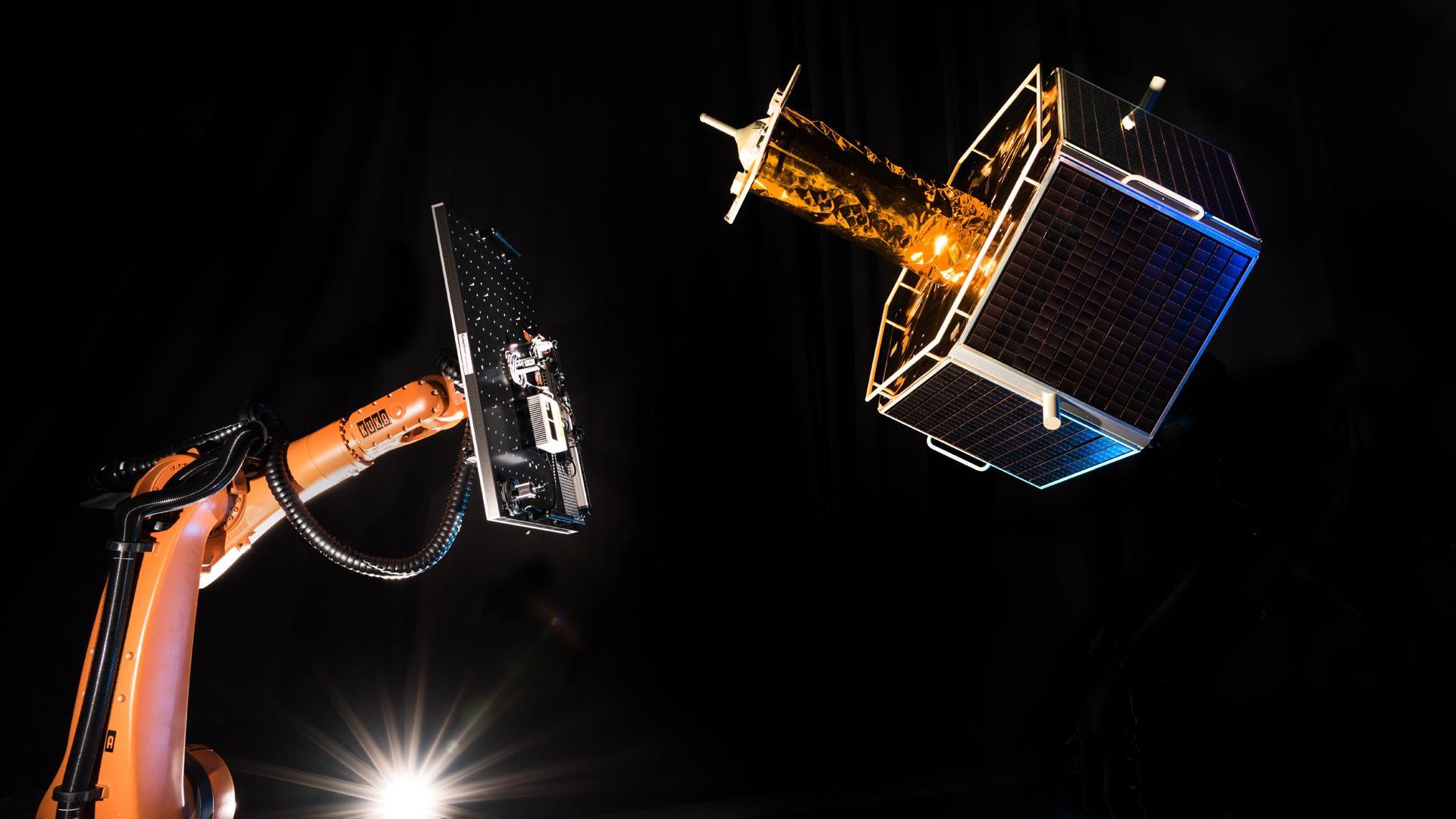
Pseudo-real images of physical spacecraft mockups in relative navigation setting and EPOS 2.0 laboratory
The intention of this research is to deploy neural-network-based relative navigation system in realistic settings after training them with synthetic images. The DLR EPOS 2.0 laboratory [Benninghoff et al., 2017] facilitates the imaging of physical scale model mockups with real cameras as well as closing the loop and using computer vision to guide and control relative navigation maneuvers. A view of the main features of the facility are given in Figure 2. The facility also features the simulation of orbit and attitude dynamics for both chaser and target spacecraft. Section “Domain randomization for sim2real and robustness” uses real images recorded during close range approach and flyby maneuvers at close range to test the performance of the segmentation-based keypoint regression network in estimating the pose of the target spacecraft.
Pose estimation using segmentation-based keypoint regression network
A full relative navigation system often requires target object position and orientation estimates to function. Without specification, ‘pose’ usually refers to both of these. A full relative navigation system usually composes of multiple components. For example, there might be a component that determines target object pose and position information without prior state information or a ‘pose initializer’. This information could then be fed to a state estimator like a Kalman filter to take advantage of the information contained in previous estimates. This work prioritizes the ‘pose initialization’ task within relative navigation systems - that is to find a pose solution from a single image without having access to previous estimates.
The full details of the utilized neural network solution is described in [Hu et al., 2019]. Only the modifications to the originally presented solution as well as a brief overview is presented in this paper to avoid repetition. The network architecture itself is unmodified compared to the reference work. The network layers are given in Figure 3. This network architecture was selected, because it was a top-scoring approach in the ESA Kelvins Spacecraft Pose Estimation competition [Kisantal et al., 2020] when evaluated on the real images of the Tango spacecraft of the PRISMA mission. This aligns with the goal of applying this network on the pseudo-real robotic laboratory images. On its input side, the network consumes a three-channel color image of size 256x256 pixels. The network outputs a 3D-tensor. Two dimensions of this tensor correspond to the 2D spatial dimensions of the image, essentially dividing the input image into a lower-resolution grid. The third dimension contains the 2D normalized image coordinates of the estimated keypoints as well as two probabilities belonging to “spacecraft” or “not spacecraft” classes. This way, each grid cell or ‘pixel’ in the output side contains its own estimate for all of the keypoints as well as the class probabilities. This means that there is a large amount of redundancy with respect to the estimates and a strategy is needed to condense these to a single set of image coordinates for each of the keypoints. In the present work, the predictions of all cells labeled “spacecraft” are used with the OpenCV implementation of EPnP [Lepetit et al., 2009] to obtain the 3D coordinates of the keypoints.

The original approach as published in [Hu et al., 2019] envisions a 3D bounding box around the target object and the corners of this project are estimated by the network. However, the solution that was used for the ESA Kelvins Pose Estimation Challenge featured a modification where the bounding box did not envelop the entire spacecraft but rather its main rectangular body, as presented by Kyle Gerard at Kelvins Day after the competition [Gerard 2019]. This was found to achieve a lower loss in training.
One aspect that has to be discussed is the applicable ranges for this network. The network learns to estimate keypoints for spacecraft that appear a certain size or at a certain range from the camera during training. This means that if during training the network has seen images taken from 3-5 meters from the target, it will not do well with an image where the target is 10 meters away from the camera, since the learned features are range-dependent. There are a couple of possible solutions to deal with this, but this work crops the spacecraft in an image based on its mask image or class label image, which means that the location of the spacecraft in the image is presumed to be known. In a full navigation system this is obviously not a realistic expectation and would therefore require a solution such as training the network on all kinds of target distances or using an object detector to crop the image. In this work it is done as a simplification to study the pose estimation pipeline’s domain adaptation characteristics and suitability for symmetric target objects.
Experiments
This section presents the experiments, their results, and the underlying reasoning for them. Network training details are not presented as they have not been changed with respect to the reference work [Hu et al., 2019], other than the loss function.
The problem of a symmetric spacecraft target
One of the immediate issues one runs into when trying to adapt the network described in section “Pose estimation using segmentation-based keypoint regression network” to the target spacecraft in Figure 4 is due to the symmetric geometry of the spacecraft. Figure 4 shows the keypoints that are estimated in the experiments in these sections. Ideally, each coordinate position in the output tensor of the neural network would always estimate the same uniquely identifiable specific fixed keypoint. However, it is clear from Figure 4 that each of the six keypoints on the main hexagonal body of the spacecraft are not uniquely identifiable as each of the six corners looks very similar to the other ones. Hexagonal corner number four wouldn’t mean anything. However, the real physical mockup spacecraft in the robotic setup and simulation of course has a unique, single pose mathematically. The problem reveals itself during training of the network - trying to adjust the weights of the network to estimate these pseudo-unique labels from simulated runs leads to the network estimating their average. The six hexagonal body keypoints as shown in Figure Figure 4 would all end up in the center of the plane they belong on as each arbitrary pseudo-unique label drags the estimates in different directions, ultimately having a loss minimum in the center of the hexagonal front plate. Essentially, one would be trying to teach the network to estimate a one-to-many relationship, which it is not set up for.
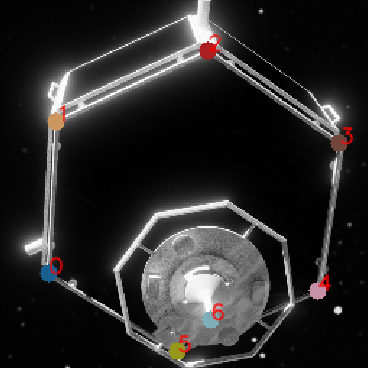
This symmetry problem can be solved if the trained problem can be reduced to a one-to-one relationship. This has been done in a simple way in Park et al., 2019, for example, where during training the closest of all of the ambiguous pose solutions is selected for loss calculations. This should pull the estimated keypoints to one of the six ambiguous pose solutions in this case, though one would not be able to control which of them. The same approach is adopted in this work, though it has to be adapted with some modifications. Since the network predicts one full set of coordinates and classes for each cell of the subgrid that the output is divided into it yields highly redundant predictions. One has two options then during training - to select the closest ambiguous pose solution for the entire group of keypoint estimates or to let each cell in the subgrid approach its own ‘closest’ solution.
Domain randomization for sim2real and robustness
Multiple principles were followed to ensure that the trained network would be able to work in all sorts of environmental and target conditions. An operational system would see a variety of lighting strengths and directions, shadows, target material and shape conditions, background, and camera settings and faults. Many of these effects are captured by varying the absolute and relative pixel intensities in the image. In this work, this has been achieved with varying some parameters inside the Blender software. The global image intensities in the image are varied via the lighting and camera parameters. The strength of the Sunlight source is varied, as well as the background texture, which also contributes to the lighting environment. Furthermore, the camera exposure time is varied. The contrast and brightness of the spacecraft are also varied via randomization of the material qualities of the shaders - the colors, metallicness, and reflectivity are randomized on all three material groups on the spacecraft model. Furthermore, a random combination of Blender’s “Magic” and “Voronoi” procedural textures are mixed in with the material representing the MLI. This is because the real physical spacecraft mockup has an MLI layer with folds and blemishes that are not represented on the model. Therefore it is not desired that the network learns to rely on the predictability of the MLI surface. The background image of a position in orbit around Earth also receives a mixing with these same random textures so that the network does not learn to separate the spacecraft purely due to the presence of these textures.
Datasets
For ease of reference, the datasets have been described and assigned unique identifiers in this section. This is to prevent confusion in the description of the experiments.
- Training dataset A: Includes 15000 images rendered with Blender. Target spacecraft rotations are random. Target range random between 5 - 30 meters. Lateral relative displacement randomn, while being limited to within 1.3 meters of the limits of the camera field of view. The largest dimension of the spacecraft is 1.32 meters from the center of rotation, so this limitation ensures the spacecraft is in full view of the camera. The direction of the Sun is randomized. The orientation of the background is randomized. The images are monochromatic.
- Training dataset B: Includes 15000 images rendered with Blender. The differences with respect to dataset A will be described. Target ranges are now not sampled uniformly with respect to distance, but rather with respect to the size of the target in the image. This is an attempt to improve accuracy at closer ranges as otherwise images where the spacecraft dominates the space of the image are underrepresented. Furthermore, multiple other factors are varied as a part of the domain randomization scheme. Additionally varied parameters include camera exposure time, background texture brightness, background and target surface texture mixing with random ‘Magic’ and ‘Voronoi’ procedural textures of Blender as well as the parameters of these textures, Sun illumination strength, target material colors, roughness, and metallicness, as well as a random gaussian blur on the images.
- Test dataset C: Includes 760 images rendered with Blender. Target spacecraft rotations cover entire pose space with 20 degree spacing in all three Euler angles. In terms of the rotation angle around symmetric axis, only a space between two ambiguous poses are covered (60 degree range due to the six-fold finite symmetry of the main hexagonal body). Target range is fixed at 5 meters and is not laterally displaced. The additional domain randomization variations present in training dataset B are not featured here. Other parameters (lighting, materials, etc) are equivalent to training dataset A.
- Test dataset D: Same as test dataset C, but at a fixed target range of 17.5 meters.
- Test dataset E: Same as test dataset C, but at a fixed target range of 30 meters.
- Test dataset F: Includes 3346 real images of a physical target spacecraft mockup from DLR EPOS 2.0 robotic close-range relative navigation laboratory at various ranges under 25 meters. Rotations and positions conform to samplings from representative approach and inspection maneuvers. Lighting conditions vary, also exhibiting some extremely overlit images. Not a lot of lateral displacement is exhibited as target is mostly centered in camera view.
Error metrics
The error metrics used in the work are unusual from the point of view of comparing neural networks performing a certain task as they are dependend on the target object, but they make sense when trying to determine the performance of this network as a part of a navigation system. The focus is on producing metrics that are intuitive for a navigation engineer.
- Longitudinal axis projection error: In the case of the target object featured in this work, there is one axis that is more important than the others. It is the symmetry axis and also the axis along which one would approach the docking adapter. This error is calculated by projecting the predicted longitudinal axis onto the ground truth longitudinal axis and extracting the angle between them via the cosine law.
- Lateral axis projection error: The error is calculated the same way as the longitudinal axis projection error, but instead an axis is used that is perpendicular to the longitudinal axis. This error expresses rotation error about the symmetry axis, which is an important quantity to estimate during the approach with the docking adapter.
- Position error magnitude: The absolute position error magnitude is also calculated to determine the quality of the position estimate.
Experiment 1
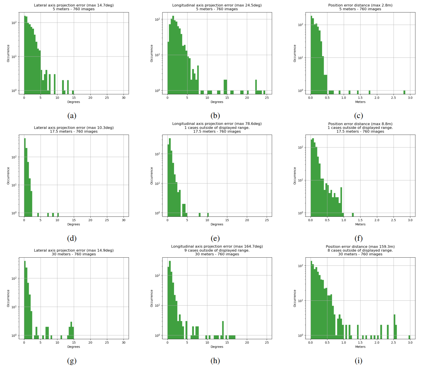
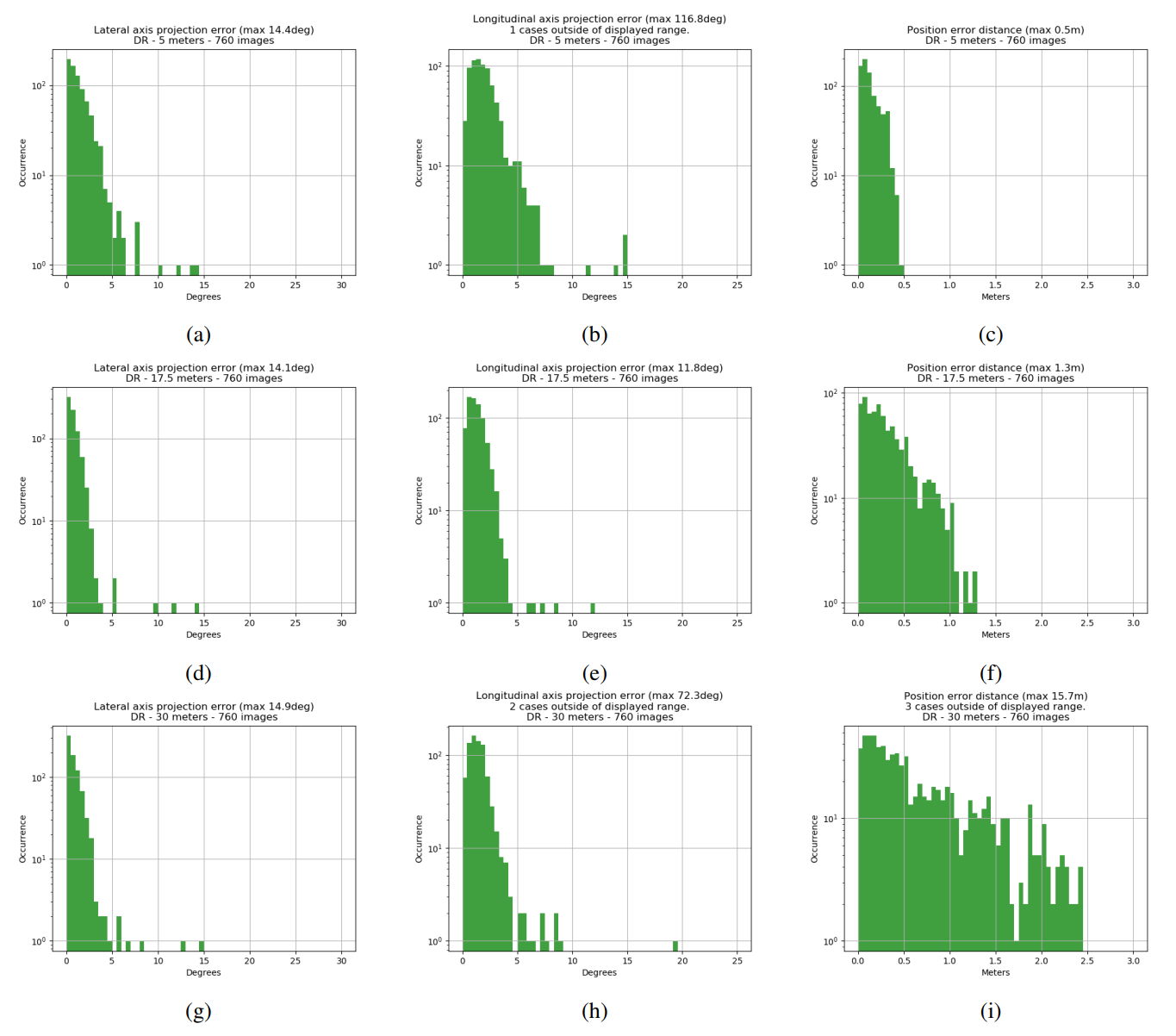
Experiment one focuses on the symmetry-adapted loss, where the entire spatial grid of the output tensor is allowed to converge on the closest ambiguous pose as a group, meaning that the average closest pose is selected for training for each individual image. The network is trained on training dataset A and tested on test datasets C, D, and E. The results of the experiment are presented in Figure 5 in terms of the metrics explained in section “Error metrics”.
The first thing to note is that the altered loss function attains meaningful results. Without it, training would collapse all points onto symmetry axis, which is unusable for any further processing. The largest angle errors occur at close range, while position error is reduced the closer the target. All graphs display “outlying” cases. Longitudinal axis error shows cases where the symmetry axis is nearly the opposite direction as to what it should be, meaning the system thinks it is looking at the back of the spacecraft when it’s looking at the front, or vice versa. This is due to a poor choice of keypoints as for the case of the observer being exactly on the symmetry axis, the keypoint locations on the image are indistinguishable between the cases of looking at the front or back of the hexagonal main body. There is a case of maximum position error of 159 meters in the 30 meter distance test set. What happens here is a failure of the PnP solver as the network predicts the keypoints correctly, but likely the PnP solver struggles to converge to either of the two ambiguous solutions caused by the chosen keypoints.
The first thing to note is that the altered loss function attains meaningful results. Without it, training would collapse all points onto symmetry axis, which is unusable for any further processing. The largest angle errors occur at close range, while position error is reduced the closer the target. All graphs display “outlying” cases. Longitudinal axis error shows cases where the symmetry axis is nearly the opposite direction as to what it should be, meaning the system thinks it is looking at the back of the spacecraft when it’s looking at the front, or vice versa. This is due to a poor choice of keypoints as for the case of the observer being exactly on the symmetry axis, the keypoint locations on the image are indistinguishable between the cases of looking at the front or back of the hexagonal main body. There is a case of maximum position error of 159 meters in the 30 meter distance test set. What happens here is a failure of the PnP solver as the network predicts the keypoints correctly, but likely the PnP solver struggles to converge to either of the two ambiguous solutions caused by the chosen keypoints.
Experiment 2
Experiment two is largely the same as the first one, except the network was trained on training dataset B, featuring domain randomization and a different sampling of target ranges, designed to make the apparent size of the target in the pictures uniformly represented in the dataset (more images at closer ranges). The results are presented in Figure 6.
The performance in terms of the angular errors has not changed in an appreciable way - at least through the lens of these histogrammed metrics. The position error has become worse at distance, but that was expected due to the lower representation of distant images in training dataset B compared to training dataset A. At least it seems that making the dataset more challenging via domain randomization has not challenged the networks too much. However, this might change with a smaller network.
Experiment 3
Experiment 3 is largely the same as experiment 2, but an even looser training loss has been used. This time, each “pixel” in the output tensor is allowed to converge to its own closest symmetric pose solution, rather than forcing them to all converge as a group towards one answer. See the results in Figure 7.
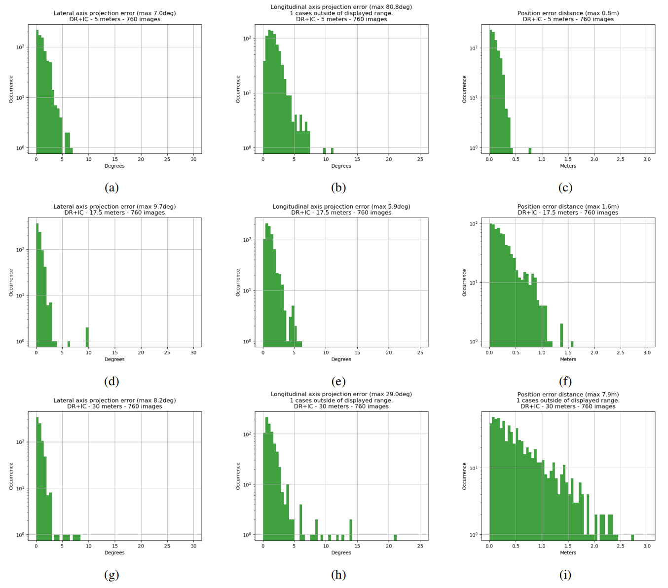
The angular error maximums decrease in all cases. Otherwise the graphs are fairly comparable.
Experiment 4
Experiment 4 is different entirely from the previous ones. The network is trained on training dataset B and evaluated on test dataset F, which is composed of real images. See the results in Figure 8
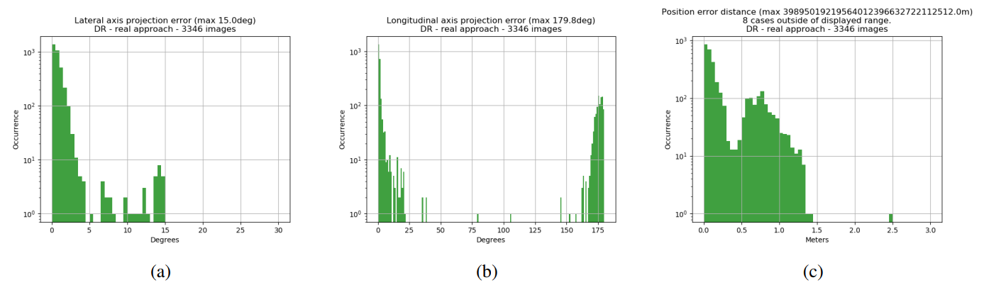
Angular error outliers and 180-degree-flips of longitudinal axis are much worse, but that is because the dataset of real images has a much higher proportion of images that are near or almost exactly on the approach/symmetry axis, which causes problems with the PnP solver. The domain randomization process has been successful in this case, as a network trained on the images of training dataset A completely failed to produce usable keypoint coordinates. They were simply spread all across the image and the network was unable to fully segment the spacecraft in the image. The network trained on domain randomized images clearly manages to make “inlying” estimates that are quite close to the error histograms of the synthetic datasets.
Dissecting outliers
Outlying pose estimates can be seen in the histograms of all experiments. However, the combined effect of domain randomization in training images and the looser loss function introduced in experiment 3 seem to have a reducing effect in terms of outliers. This section will explore some of the outlying cases that remain in experiment 3 as well as the ones in experiment 4.
The dataset of real images of experiment 4 reveal a couple of failure modes. The first failure mode is to do with the keypoint estimates from the neural network not agreeing on which symmetrically ambiguous pose to estimate. Often the keypoints passed to the PnP solver in a failure mode like this still manage to produce a fairly accurate pose. The other failure mode originates from the choice of keypoints on the spacecraft. At certain attitudes of the spacecraft, they project onto the image in a way that is ambiguous when one tries to go from 2D to 3D again with the PnP-solver. Most importantly, this happens in the approach direction. When the chaser is aligned with the symmetry axis on approach, the keypoints in the image could belong to a pose where the chaser is approaching the docking adapter or where the chaser is looking at the back of the hexagonal main body. In addition to these failures, the synthetic datasets feature a few more situations where the keypoint projections cause the PnP-solver to settle on the wrong answer.
References
[Sharma et al. 2016] S. Sharma, S. D׳Amico, Comparative assessment of techniques for initial pose estimation using monocular vision, Acta Astronautica, Volume 123, 2016, Pages 435-445, doi: 10.1016/j.actaastro.2015.12.032
[Sharma et al. 2018] S. Sharma, C. Beierle and S. D’Amico, Pose estimation for non-cooperative spacecraft rendezvous using convolutional neural networks, 2018 IEEE Aerospace Conference, 2018, Pages 1-12, doi: 10.1109/AERO.2018.8396425
[Kisantal et al. 2020] M. Kisantal, S. Sharma, T.H. Park, D. Izzo, M. Märtens, and S. D’Amico, Satellite Pose Estimation Challenge: Dataset, Competition Design, and Results, IEEE Transactions on Aerospace and Electronic Systems, Volume 56, 2020, Pages 4083-4098, doi: 10.1109/TAES.2020.2989063
[Kehl et al. 2017] W. Kehl, F. Manhardt, F. Tombari, S. Ilic, and N. Navab, SSD-6D: Making RGB-Based 3D Detection and 6D Pose Estimation Great Again, 2017 IEEE International Conference on Computer Vision (ICCV), 2017, Pages 1530-1538, doi: 10.1109/ICCV.2017.169
[Rad et al. 2017] M. Rad and V. Lepetit, BB8: A Scalable, Accurate, Robust to Partial Occlusion Method for Predicting the 3D Poses of Challenging Objects without Using Depth, 2017 IEEE International Conference on Computer Vision (ICCV), 2017, Pages 3848-3856, doi: 10.1109/ICCV.2017.413
[Corona et al. 2018] E. Corona, K. Kundu and S. Fidler, Pose Estimation for Objects with Rotational Symmetry, 2018 IEEE/RSJ International Conference on Intelligent Robots and Systems (IROS), 2018, Pages 7215-7222, doi: 10.1109/IROS.2018.8594282
[Xiang et al. 2018] Y. Xiang, T. Schmidt, V. Narayanan, and D. Fox, PoseCNN: A Convolutional Neural Network for 6D Object Pose Estimation in Cluttered Scenes, Robotics: Science and Systems 2018, 2018, doi: 10.15607/RSS.2018.XIV.019
[Sundermeyer et al. 2018] M. Sundermeyer, Z.C. Marton, M. Durner, M. Brucker, and R. Triebel, Implicit 3D Orientation Learning for 6D Object Detection from RGB Images, The European Conference on Computer Vision (ECCV), 2018
[Park et al. 2019] K. Park, T. Patten and M. Vincze, Pix2Pose: Pixel-Wise Coordinate Regression of Objects for 6D Pose Estimation, 2019 IEEE/CVF International Conference on Computer Vision (ICCV), 2019, Pages 7667-7676, doi: 10.1109/ICCV.2019.00776
[Manhardt et al. 2019] F. Manhardt, D.M. Arroyo, C. Rupprecht, B. Busam, T. Birdal, N. Navab, and F. Tombari, Explaining the Ambiguity of Object Detection and 6D Pose From Visual Data, 2019 IEEE/CVF International Conference on Computer Vision (ICCV), 2019, Pages 6840-6849, doi: 10.1109/ICCV.2019.00694
[Hodan et al. 2020]
T. Hodan, D. Barath and J. Matas,
EPOS: Estimating 6D Pose of Objects With Symmetries,
2020 IEEE/CVF Conference on Computer Vision and Pattern Recognition (CVPR), 2020,
Pages 11700-11709,
doi: 10.1109/CVPR42600.2020.01172
[Hu et al. 2019] Y. Hu, J. Hugonot, P. Fua and M. Salzmann, Segmentation-Driven 6D Object Pose Estimation, 2019 IEEE/CVF Conference on Computer Vision and Pattern Recognition (CVPR), 2019, Pages 3380-3389, doi: 10.1109/CVPR.2019.00350
[Gerard 2019] Kyle Gerard, Segmentation-driven Satellite Pose Estimation, Kelvins Day 2019, 2019
[Kajak et al. 2021] K.M. Kajak, C. Maddock, H. Frei, K. Schwenk, Segmentation-driven spacecraft pose estimation for vision-based relative navigation in space, 72nd International Astronautical Congress, 2021
[Opiela 2009] J.N. Opiela, A study of the material density distribution of space debris, Advances in Space Research, Volume 43, Issue 7, 2009, Pages 1058-1064, doi: 10.1016/j.asr.2008.12.013
[Benninghoff et al. 2017] H. Benninghoff, F. Rems, E.A. Risse, and C. Mietner, European Proximity Operations Simulator 2.0 (EPOS) - A Robotic-Based Rendezvous and Docking Simulator, Journal of large-scale research facilities, 3, A107, 2017, doi: 10.17815/jlsrf-3-155
[Lepetit et al. 2009] V. Lepetit, F. Moreno-Noguer, and P. Fua, EPnP: An Accurate O(n) Solution to the PnP Problem, International Journal of Computer Vision 81, article #155, 2009, doi: 10.1007/s11263-008-0152-6
[Rathinam et al. 2020] A. Rathinam, Y, Gao, On-Orbit Relative Navigation Near a Known Target Using Monocular Vision and Convolutional Neural Networks for Pose Estimation, International Symposium on Artificial Intelligence, Robotics and Automation in Space (iSAIRAS), 2020
[Cheng et al. 2020] B. Cheng, B. Xiao, J. Wang, H. Shi, T. S. Huang and L. Zhang, HigherHRNet: Scale-Aware Representation Learning for Bottom-Up Human Pose Estimation, 2020 IEEE/CVF Conference on Computer Vision and Pattern Recognition (CVPR), 2020, Pages 5385-5394, doi: 10.1109/CVPR42600.2020.00543